Descriptive statistics and inferential statistics are both important components of statistics when learning about a population.
Learning Objective
Contrast descriptive and inferential statistics
Key Points
Descriptive statistics are distinguished from inferential statistics in that descriptive statistics aim to summarize a sample, rather than use the data to learn about the population that the sample of data is thought to represent.
Descriptive statistics provides simple summaries about the sample. These summaries may either form the basis of the initial description of the data as part of a more extensive statistical analysis, or they may be sufficient in and of themselves for a particular investigation.
Statistical inference makes propositions about populations, using data drawn from the population of interest via some form of random sampling. This involves hypothesis testing using a variety of statistical tests.
Key Terms
descriptive statistics
A branch of mathematics dealing with summarization and description of collections of data sets, including the concepts of arithmetic mean, median, and mode.
inferential statistics
A branch of mathematics that involves drawing conclusions about a population based on sample data drawn from it.
Descriptive Statistics vs. Inferential Statistics
Descriptive statistics is the discipline of quantitatively describing the main features of a collection of data, or the quantitative description itself. Descriptive statistics are distinguished from inferential statistics in that descriptive statistics aim to summarize a sample, rather than use the data to learn about the population that the sample of data is thought to represent. This generally means that descriptive statistics, unlike inferential statistics, are not developed on the basis of probability theory. Even when a data analysis draws its main conclusions using inferential statistics, descriptive statistics are generally also presented. For example, in a paper reporting on a study involving human subjects, there typically appears a table giving the overall sample size, sample sizes in important subgroups (e.g., for each treatment or exposure group), and demographic or clinical characteristics such as the average age and the proportion of subjects of each sex.
Descriptive Statistics
Descriptive statistics provides simple summaries about the sample and about the observations that have been made. Such summaries may be either quantitative, i.e. summary statistics, or visual, i.e. simple-to-understand graphs. These summaries may either form the basis of the initial description of the data as part of a more extensive statistical analysis, or they may be sufficient in and of themselves for a particular investigation.
For example, the shooting percentage in basketball is a descriptive statistic that summarizes the performance of a player or a team. This number is the number of shots made divided by the number of shots taken. For example, a player who shoots 33% is making approximately one shot in every three. The percentage summarizes or describes multiple discrete events. Consider also the grade point average. This single number describes the general performance of a student across the range of their course experiences.
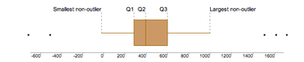
The use of descriptive and summary statistics has an extensive history and, indeed, the simple tabulation of populations and of economic data was the first way the topic of statistics appeared. More recently, a collection of summary techniques has been formulated under the heading of exploratory data analysis: an example of such a technique is the box plot .
Box Plot
The box plot is a graphical depiction of descriptive statistics.
In the business world, descriptive statistics provide a useful summary of security returns when researchers perform empirical and analytical analysis, as they give a historical account of return behavior.
Inferential Statistics
For the most part, statistical inference makes propositions about populations, using data drawn from the population of interest via some form of random sampling. More generally, data about a random process is obtained from its observed behavior during a finite period of time. Given a parameter or hypothesis about which one wishes to make inference, statistical inference most often uses a statistical model of the random process that is supposed to generate the data and a particular realization of the random process.
The conclusion of a statistical inference is a statistical proposition. Some common forms of statistical proposition are:
an estimate; i.e., a particular value that best approximates some parameter of interest
a confidence interval (or set estimate); i.e., an interval constructed using a data set drawn from a population so that, under repeated sampling of such data sets, such intervals would contain the true parameter value with the probability at the stated confidence level
a credible interval; i.e., a set of values containing, for example, 95% of posterior belief
rejection of a hypothesis
clustering or classification of data points into groups
14.1.2: Hypothesis Tests or Confidence Intervals?
Hypothesis tests and confidence intervals are related, but have some important differences.
Learning Objective
Explain how confidence intervals are used to estimate parameters of interest
Key Points
When we conduct a hypothesis test, we assume we know the true parameters of interest.
When we use confidence intervals, we are estimating the the parameters of interest.
The confidence interval for a parameter is not the same as the acceptance region of a test for this parameter, as is sometimes thought.
The confidence interval is part of the parameter space, whereas the acceptance region is part of the sample space.
Key Terms
hypothesis test
A test that defines a procedure that controls the probability of incorrectly deciding that a default position (null hypothesis) is incorrect based on how likely it would be for a set of observations to occur if the null hypothesis were true.
confidence interval
A type of interval estimate of a population parameter used to indicate the reliability of an estimate.
What is the difference between hypothesis testing and confidence intervals? When we conduct a hypothesis test, we assume we know the true parameters of interest. When we use confidence intervals, we are estimating the parameters of interest.
Explanation of the Difference
Confidence intervals are closely related to statistical significance testing. For example, if for some estimated parameter
one wants to test the null hypothesis that
against the alternative that
, then this test can be performed by determining whether the confidence interval for
contains
.
More generally, given the availability of a hypothesis testing procedure that can test the null hypothesis
against the alternative that
for any value of
, then a confidence interval with confidence level
can be defined as containing any number
for which the corresponding null hypothesis is not rejected at significance level
.
In consequence, if the estimates of two parameters (for example, the mean values of a variable in two independent groups of objects) have confidence intervals at a given
value that do not overlap, then the difference between the two values is significant at the corresponding value of
. However, this test is too conservative. If two confidence intervals overlap, the difference between the two means still may be significantly different.
While the formulations of the notions of confidence intervals and of statistical hypothesis testing are distinct, in some senses and they are related, and are complementary to some extent. While not all confidence intervals are constructed in this way, one general purpose approach is to define a
% confidence interval to consist of all those values
for which a test of the hypothesis
is not rejected at a significance level of
%. Such an approach may not always be an option, since it presupposes the practical availability of an appropriate significance test. Naturally, any assumptions required for the significance test would carry over to the confidence intervals.
It may be convenient to say that parameter values within a confidence interval are equivalent to those values that would not be rejected by a hypothesis test, but this would be dangerous. In many instances the confidence intervals that are quoted are only approximately valid, perhaps derived from “plus or minus twice the standard error,” and the implications of this for the supposedly corresponding hypothesis tests are usually unknown.
It is worth noting that the confidence interval for a parameter is not the same as the acceptance region of a test for this parameter, as is sometimes assumed. The confidence interval is part of the parameter space, whereas the acceptance region is part of the sample space. For the same reason, the confidence level is not the same as the complementary probability of the level of significance.
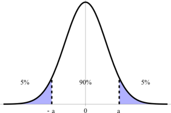
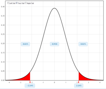
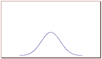
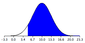
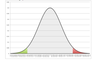
Confidence Interval
This graph illustrates a 90% confidence interval on a standard normal curve.
14.1.3: Quantitative or Qualitative Data?
Different statistical tests are used to test quantitative and qualitative data.
Learning Objective
Contrast quantitative and qualitative data
Key Points
Quantitative (numerical) data is any data that is in numerical form, such as statistics and percentages.
Qualitative (categorical) data deals with descriptions with words, such as gender or nationality.
Paired and unpaired t-tests and z-tests are just some of the statistical tests that can be used to test quantitative data.
One of the most common statistical tests for qualitative data is the chi-square test (both the goodness of fit test and test of independence).
Key Terms
central limit theorem
The theorem that states: If the sum of independent identically distributed random variables has a finite variance, then it will be (approximately) normally distributed.
quantitative
of a measurement based on some quantity or number rather than on some quality
qualitative
of descriptions or distinctions based on some quality rather than on some quantity
Quantitative Data vs. Qualitative Data
Recall the differences between quantitative and qualitative data.
Quantitative (numerical) data is any data that is in numerical form, such as statistics, percentages, et cetera. In layman’s terms, a researcher studying quantitative data asks a specific, narrow question and collects a sample of numerical data from participants to answer the question. The researcher analyzes the data with the help of statistics and hopes the numbers will yield an unbiased result that can be generalized to some larger population.
Qualitative (categorical) research, on the other hand, asks broad questions and collects word data from participants. The researcher looks for themes and describes the information in themes and patterns exclusive to that set of participants. Examples of qualitative variables are male/female, nationality, color, et cetera.
Quantitative Data Tests
Paired and unpaired t-tests and z-tests are just some of the statistical tests that can be used to test quantitative data. We will give a brief overview of these tests here.
A t-test is any statistical hypothesis test in which the test statistic follows a t distribution if the null hypothesis is supported. It can be used to determine if two sets of data are significantly different from each other and is most commonly applied when the test statistic would follow a normal distribution if the value of a scaling term in the test statistic were known. When the scaling term is unknown and is replaced by an estimate based on the data, the test statistic (under certain conditions) follows a t distribution .
t Distribution
Plots of the t distribution for several different degrees of freedom.
A z-test is any statistical test for which the distribution of the test statistic under the null hypothesis can be approximated by a normal distribution. Because of the central limit theorem, many test statistics are approximately normally distributed for large samples. For each significance level, the z-test has a single critical value. This fact makes it more convenient than the t-test, which has separate critical values for each sample size. Therefore, many statistical tests can be conveniently performed as approximate z-tests if the sample size is large or the population variance known.
Qualitative Data Tests
One of the most common statistical tests for qualitative data is the chi-square test (both the goodness of fit test and test of independence).
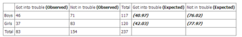
The chi-square test tests a null hypothesis stating that the frequency distribution of certain events observed in a sample is consistent with a particular theoretical distribution. The events considered must be mutually exclusive and have total probability. A common case for this test is where the events each cover an outcome of a categorical variable. A test of goodness of fit establishes whether or not an observed frequency distribution differs from a theoretical distribution, and a test of independence assesses whether paired observations on two variables, expressed in a contingency table, are independent of each other (e.g., polling responses from people of different nationalities to see if one’s nationality is related to the response).
14.1.4: One, Two, or More Groups?
Different statistical tests are required when there are different numbers of groups (or samples).
Learning Objective
Identify the appropriate statistical test required for a group of samples
Key Points
One-sample tests are appropriate when a sample is being compared to the population from a hypothesis. The population characteristics are known from theory or are calculated from the population.
Two-sample tests are appropriate for comparing two samples, typically experimental and control samples from a scientifically controlled experiment.
Paired tests are appropriate for comparing two samples where it is impossible to control important variables.
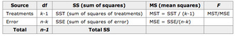
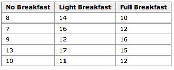
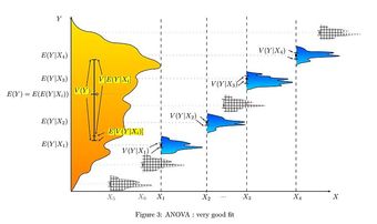
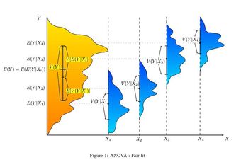
-tests (analysis of variance, also called ANOVA) are used when there are more than two groups. They are commonly used when deciding whether groupings of data by category are meaningful.
Key Terms
z-test
Any statistical test for which the distribution of the test statistic under the null hypothesis can be approximated by a normal distribution.
t-test
Any statistical hypothesis test in which the test statistic follows a Student’s $t$-distribution if the null hypothesis is supported.
Depending on how many groups (or samples) with which we are working, different statistical tests are required.
One-sample tests are appropriate when a sample is being compared to the population from a hypothesis. The population characteristics are known from theory, or are calculated from the population. Two-sample tests are appropriate for comparing two samples, typically experimental and control samples from a scientifically controlled experiment. Paired tests are appropriate for comparing two samples where it is impossible to control important variables. Rather than comparing two sets, members are paired between samples so the difference between the members becomes the sample. Typically the mean of the differences is then compared to zero.
The number of groups or samples is also an important deciding factor when determining which test statistic is appropriate for a particular hypothesis test. A test statistic is considered to be a numerical summary of a data-set that reduces the data to one value that can be used to perform a hypothesis test. Examples of test statistics include the
-statistic,
-statistic, chi-square statistic, and
-statistic.
A
-statistic may be used for comparing one or two samples or proportions. When comparing two proportions, it is necessary to use a pooled standard deviation for the
-test. The formula to calculate a
-statistic for use in a one-sample
-test is as follows:
where
is the sample mean,
is the population mean,
is the population standard deviation, and
is the sample size.
A
-statistic may be used for one sample, two samples (with a pooled or unpooled standard deviation), or for a regression
-test. The formula to calculate a
-statistic for a one-sample
-test is as follows:
where
is the sample mean,
is the population mean,
is the sample standard deviation, and
is the sample size.
-tests (analysis of variance, also called ANOVA) are used when there are more than two groups. They are commonly used when deciding whether groupings of data by category are meaningful. If the variance of test scores of the left-handed in a class is much smaller than the variance of the whole class, then it may be useful to study lefties as a group. The null hypothesis is that two variances are the same, so the proposed grouping is not meaningful.
14.2: A Closer Look at Tests of Significance
14.2.1: Was the Result Significant?
Results are deemed significant if they are found to have occurred by some reason other than chance.
Learning Objective
Assess the statistical significance of data for a null hypothesis
Key Points
In statistical testing, a result is deemed statistically significant if it is so extreme (without external variables which would influence the correlation results of the test) that such a result would be expected to arise simply by chance only in rare circumstances.
If a test of significance gives a p-value lower than or equal to the significance level, the null hypothesis is rejected at that level.
Different levels of cutoff trade off countervailing effects. Lower levels – such as 0.01 instead of 0.05 – are stricter, and increase confidence in the determination of significance, but run an increased risk of failing to reject a false null hypothesis.
Key Terms
statistical significance
A measure of how unlikely it is that a result has occurred by chance.
null hypothesis
A hypothesis set up to be refuted in order to support an alternative hypothesis; presumed true until statistical evidence in the form of a hypothesis test indicates otherwise.
Statistical significance refers to two separate notions: the p-value (the probability that the observed data would occur by chance in a given single null hypothesis); or the Type I error rate α (false positive rate) of a statistical hypothesis test (the probability of incorrectly rejecting a given null hypothesis in favor of a second alternative hypothesis).
A fixed number, most often 0.05, is referred to as a significance level or level of significance; such a number may be used either in the first sense, as a cutoff mark for p-values (each p-value is calculated from the data), or in the second sense as a desired parameter in the test design (α depends only on the test design, and is not calculated from observed data). In this atom, we will focus on the p-value notion of significance.
What is Statistical Significance?
Statistical significance is a statistical assessment of whether observations reflect a pattern rather than just chance. When used in statistics, the word significant does not mean important or meaningful, as it does in everyday speech; with sufficient data, a statistically significant result may be very small in magnitude.
The fundamental challenge is that any partial picture of a given hypothesis, poll, or question is subject to random error. In statistical testing, a result is deemed statistically significant if it is so extreme (without external variables which would influence the correlation results of the test) that such a result would be expected to arise simply by chance only in rare circumstances. Hence the result provides enough evidence to reject the hypothesis of ‘no effect’.
For example, tossing 3 coins and obtaining 3 heads would not be considered an extreme result. However, tossing 10 coins and finding that all 10 land the same way up would be considered an extreme result: for fair coins, the probability of having the first coin matched by all 9 others is rare. The result may therefore be considered statistically significant evidence that the coins are not fair.
The calculated statistical significance of a result is in principle only valid if the hypothesis was specified before any data were examined. If, instead, the hypothesis was specified after some of the data were examined, and specifically tuned to match the direction in which the early data appeared to point, the calculation would overestimate statistical significance.
Use in Practice
Popular levels of significance are 10% (0.1), 5% (0.05), 1% (0.01), 0.5% (0.005), and 0.1% (0.001). If a test of significance gives a p-value lower than or equal to the significance level , the null hypothesis is rejected at that level. Such results are informally referred to as ‘statistically significant (at the p = 0.05 level, etc.)’. For example, if someone argues that “there’s only one chance in a thousand this could have happened by coincidence”, a 0.001 level of statistical significance is being stated. The lower the significance level chosen, the stronger the evidence required. The choice of significance level is somewhat arbitrary, but for many applications, a level of 5% is chosen by convention.
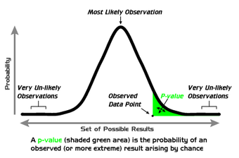
P-Values
A graphical depiction of the meaning of p-values.
Different levels of cutoff trade off countervailing effects. Lower levels – such as 0.01 instead of 0.05 – are stricter, and increase confidence in the determination of significance, but run an increased risk of failing to reject a false null hypothesis. Evaluation of a given p-value of data requires a degree of judgment, and rather than a strict cutoff, one may instead simply consider lower p-values as more significant.
14.2.2: Data Snooping: Testing Hypotheses Once You’ve Seen the Data
Testing hypothesis once you’ve seen the data may result in inaccurate conclusions.
Learning Objective
Explain how to test a hypothesis using data
Key Points
Testing a hypothesis suggested by the data can very easily result in false positives (type I errors). If one looks long enough and in enough different places, eventually data can be found to support any hypothesis.
If the hypothesis was specified after some of the data were examined, and specifically tuned to match the direction in which the early data appeared to point, the calculation would overestimate statistical significance.
Sometimes, people deliberately test hypotheses once they’ve seen the data. Data snooping (also called data fishing or data dredging) is the inappropriate (sometimes deliberately so) use of data mining to uncover misleading relationships in data.
Key Terms
Type I error
Rejecting the null hypothesis when the null hypothesis is true.
data snooping
the inappropriate (sometimes deliberately so) use of data mining to uncover misleading relationships in data
The calculated statistical significance of a result is in principle only valid if the hypothesis was specified before any data were examined. If, instead, the hypothesis was specified after some of the data were examined, and specifically tuned to match the direction in which the early data appeared to point, the calculation would overestimate statistical significance.
Testing Hypotheses Suggested by the Data
Testing a hypothesis suggested by the data can very easily result in false positives (type I errors) . If one looks long enough and in enough different places, eventually data can be found to support any hypothesis. Unfortunately, these positive data do not by themselves constitute evidence that the hypothesis is correct. The negative test data that were thrown out are just as important, because they give one an idea of how common the positive results are compared to chance. Running an experiment, seeing a pattern in the data, proposing a hypothesis from that pattern, then using the same experimental data as evidence for the new hypothesis is extremely suspect, because data from all other experiments, completed or potential, has essentially been “thrown out” by choosing to look only at the experiments that suggested the new hypothesis in the first place.
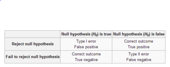
Types of Errors
This table depicts the difference types of errors in significance testing.
A large set of tests as described above greatly inflates the probability of type I error as all but the data most favorable to the hypothesis is discarded. This is a risk, not only in hypothesis testing but in all statistical inference as it is often problematic to accurately describe the process that has been followed in searching and discarding data. In other words, one wants to keep all data (regardless of whether they tend to support or refute the hypothesis) from “good tests”, but it is sometimes difficult to figure out what a “good test” is. It is a particular problem in statistical modelling, where many different models are rejected by trial and error before publishing a result.
The error is particularly prevalent in data mining and machine learning. It also commonly occurs in academic publishing where only reports of positive, rather than negative, results tend to be accepted, resulting in the effect known as publication bias..
Data Snooping
Sometimes, people deliberately test hypotheses once they’ve seen the data. Data snooping (also called data fishing or data dredging) is the inappropriate (sometimes deliberately so) use of data mining to uncover misleading relationships in data. Data-snooping bias is a form of statistical bias that arises from this misuse of statistics. Any relationships found might appear valid within the test set but they would have no statistical significance in the wider population. Although data-snooping bias can occur in any field that uses data mining, it is of particular concern in finance and medical research, which both heavily use data mining.
14.2.3: Was the Result Important?
The results are deemed important if they change the effects of an event.
Learning Objective
Distinguish the difference between the terms ‘significance’ and ‘importance’ in statistical assessments
Key Points
When used in statistics, the word significant does not mean important or meaningful, as it does in everyday speech; with sufficient data, a statistically significant result may be very small in magnitude.
Importance is a measure of the effects of the event. A difference can be significant, but not important.
It is preferable for researchers to not look solely at significance, but to examine effect-size statistics, which describe how large the effect is and the uncertainty around that estimate, so that the practical importance of the effect may be gauged by the reader.
Key Terms
null hypothesis
A hypothesis set up to be refuted in order to support an alternative hypothesis; presumed true until statistical evidence in the form of a hypothesis test indicates otherwise.
statistical significance
A measure of how unlikely it is that a result has occurred by chance.
Significance vs. Importance
Statistical significance is a statistical assessment of whether observations reflect a pattern rather than just chance. When used in statistics, the word significant does not mean important or meaningful, as it does in everyday speech; with sufficient data, a statistically significant result may be very small in magnitude.
If a test of significance gives a
-value lower than or equal to the significance level, the null hypothesis is rejected at that level . Such results are informally referred to as ‘statistically significant (at the
level, etc.)’. For example, if someone argues that “there’s only one chance in a thousand this could have happened by coincidence”, a
level of statistical significance is being stated. Once again, this does not mean that the findings are important.
-Values
A graphical depiction of the meaning of
-values.
So what is importance? Importance is a measure of the effects of the event. For example, we could measure two different one-cup measuring cups enough times to find that their volumes are statistically different at a significance level of
. But is this difference important? Would this slight difference make a difference in the cookies you’re trying to bake? No. The difference in this case is statistically significant at a certain level, but not important.
Researchers focusing solely on whether individual test results are significant or not may miss important response patterns which individually fall under the threshold set for tests of significance. Therefore along with tests of significance, it is preferable to examine effect-size statistics, which describe how large the effect is and the uncertainty around that estimate, so that the practical importance of the effect may be gauged by the reader.
14.2.4: The Role of the Model
A statistical model is a set of assumptions concerning the generation of the observed data and similar data.
Learning Objective
Explain the significance of valid models in statistical inference
Key Points
Statisticians distinguish between three levels of modeling assumptions: fully-parametric, non-parametric, and semi-parametric.
Descriptions of statistical models usually emphasize the role of population quantities of interest, about which we wish to draw inference. Descriptive statistics are typically used as a preliminary step before more formal inferences are drawn.
Whatever level of assumption is made, correctly calibrated inference in general requires these assumptions to be correct; i.e., that the data-generating mechanisms have been correctly specified.
Key Terms
Simple Random Sampling
Method where each individual is chosen randomly and entirely by chance, such that each individual has the same probability of being chosen at any stage during the sampling process, and each subset of k individuals has the same probability of being chosen for the sample as any other subset of k individuals.
covariate
a variable that is possibly predictive of the outcome under study
Any statistical inference requires assumptions. A statistical model is a set of assumptions concerning the generation of the observed data and similar data. Descriptions of statistical models usually emphasize the role of population quantities of interest, about which we wish to draw inference. Descriptive statistics are typically used as a preliminary step before more formal inferences are drawn.
Degrees of Models
Statisticians distinguish between three levels of modeling assumptions:
Fully-parametric. The probability distributions describing the data-generation process are assumed to be fully described by a family of probability distributions involving only a finite number of unknown parameters. For example, one may assume that the distribution of population values is truly Normal , with unknown mean and variance, and that data sets are generated by simple random sampling. The family of generalized linear models is a widely used and flexible class of parametric models.
Non-parametric. The assumptions made about the process generating the data are much fewer than in parametric statistics and may be minimal. For example, every continuous probability distribution has a median that may be estimated using the sample median, which has good properties when the data arise from simple random sampling.
Semi-parametric. This term typically implies assumptions in between fully and non-parametric approaches. For example, one may assume that a population distribution has a finite mean. Furthermore, one may assume that the mean response level in the population depends in a truly linear manner on some covariate (a parametric assumption), but not make any parametric assumption describing the variance around that mean. More generally, semi-parametric models can often be separated into ‘structural’ and ‘random variation’ components. One component is treated parametrically and the other non-parametrically.
Importance of Valid Models
Whatever level of assumption is made, correctly calibrated inference in general requires these assumptions to be correct (i.e., that the data-generating mechanisms have been correctly specified).
Incorrect assumptions of simple random sampling can invalidate statistical inference. More complex semi- and fully parametric assumptions are also cause for concern. For example, incorrect “Assumptions of Normality” in the population invalidate some forms of regression-based inference. The use of any parametric model is viewed skeptically by most experts in sampling human populations. In particular, a normal distribution would be a totally unrealistic and unwise assumption to make if we were dealing with any kind of economic population. Here, the central limit theorem states that the distribution of the sample mean for very large samples is approximately normally distributed, if the distribution is not heavy tailed.
14.2.5: Does the Difference Prove the Point?
Rejecting the null hypothesis does not necessarily prove the alternative hypothesis.
Learning Objective
Assess whether a null hypothesis should be accepted or rejected
Key Points
The “fail to reject” terminology highlights the fact that the null hypothesis is assumed to be true from the start of the test; therefore, if there is a lack of evidence against it, it simply continues to be assumed true.
The phrase “accept the null hypothesis” may suggest it has been proven simply because it has not been disproved, a logical fallacy known as the argument from ignorance.
Unless a test with particularly high power is used, the idea of “accepting” the null hypothesis may be dangerous.
Whether rejection of the null hypothesis truly justifies acceptance of the alternative hypothesis depends on the structure of the hypotheses.
Hypothesis testing emphasizes the rejection, which is based on a probability, rather than the acceptance, which requires extra steps of logic.
Key Terms
null hypothesis
A hypothesis set up to be refuted in order to support an alternative hypothesis; presumed true until statistical evidence in the form of a hypothesis test indicates otherwise.
p-value
The probability of obtaining a test statistic at least as extreme as the one that was actually observed, assuming that the null hypothesis is true.
alternative hypothesis
a rival hypothesis to the null hypothesis, whose likelihoods are compared by a statistical hypothesis test
In statistical hypothesis testing, tests are used in determining what outcomes of a study would lead to a rejection of the null hypothesis for a pre-specified level of significance; this can help to decide whether results contain enough information to cast doubt on conventional wisdom, given that conventional wisdom has been used to establish the null hypothesis. The critical region of a hypothesis test is the set of all outcomes which cause the null hypothesis to be rejected in favor of the alternative hypothesis.
Accepting the Null Hypothesis vs. Failing to Reject It
It is important to note the philosophical difference between accepting the null hypothesis and simply failing to reject it. The “fail to reject” terminology highlights the fact that the null hypothesis is assumed to be true from the start of the test; if there is a lack of evidence against it, it simply continues to be assumed true. The phrase “accept the null hypothesis” may suggest it has been proved simply because it has not been disproved, a logical fallacy known as the argument from ignorance. Unless a test with particularly high power is used, the idea of “accepting” the null hypothesis may be dangerous. Nonetheless, the terminology is prevalent throughout statistics, where its meaning is well understood.
Alternatively, if the testing procedure forces us to reject the null hypothesis (
), we can accept the alternative hypothesis (
) and we conclude that the research hypothesis is supported by the data. This fact expresses that our procedure is based on probabilistic considerations in the sense we accept that using another set of data could lead us to a different conclusion.
What Does This Mean?
If the
-value is less than the required significance level (equivalently, if the observed test statistic is in the critical region), then we say the null hypothesis is rejected at the given level of significance. Rejection of the null hypothesis is a conclusion. This is like a “guilty” verdict in a criminal trial—the evidence is sufficient to reject innocence, thus proving guilt. We might accept the alternative hypothesis (and the research hypothesis).
-Values
A graphical depiction of the meaning of
-values.
If the
-value is not less than the required significance level (equivalently, if the observed test statistic is outside the critical region), then the test has no result. The evidence is insufficient to support a conclusion. This is like a jury that fails to reach a verdict. The researcher typically gives extra consideration to those cases where the
-value is close to the significance level.
Whether rejection of the null hypothesis truly justifies acceptance of the research hypothesis depends on the structure of the hypotheses. Rejecting the hypothesis that a large paw print originated from a bear does not immediately prove the existence of Bigfoot. The two hypotheses in this case are not exhaustive; there are other possibilities. Maybe a moose made the footprints. Hypothesis testing emphasizes the rejection which is based on a probability rather than the acceptance which requires extra steps of logic.
A t-test is any statistical hypothesis test in which the test statistic follows a Student’s t-distribution if the null hypothesis is supported.
Learning Objective
Outline the appropriate uses of t-tests in Student’s t-distribution
Key Points
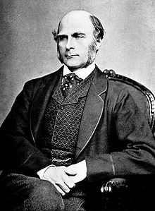
The t-statistic was introduced in 1908 by William Sealy Gosset, a chemist working for the Guinness brewery in Dublin, Ireland.
The t-test can be used to determine if two sets of data are significantly different from each other.
The t-test is most commonly applied when the test statistic would follow a normal distribution if the value of a scaling term in the test statistic were known.
Key Terms
t-test
Any statistical hypothesis test in which the test statistic follows a Student’s t-distribution if the null hypothesis is supported.
Student’s t-distribution
A family of continuous probability distributions that arises when estimating the mean of a normally distributed population in situations where the sample size is small and population standard deviation is unknown.
A t-test is any statistical hypothesis test in which the test statistic follows a Student’s t-distribution if the null hypothesis is supported. It can be used to determine if two sets of data are significantly different from each other, and is most commonly applied when the test statistic would follow a normal distribution if the value of a scaling term in the test statistic were known. When the scaling term is unknown and is replaced by an estimate based on the data, the test statistic (under certain conditions) follows a Student’s t-distribution.
History
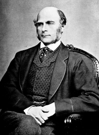
The t-statistic was introduced in 1908 by William Sealy Gosset (shown in ), a chemist working for the Guinness brewery in Dublin, Ireland. Gosset had been hired due to Claude Guinness’s policy of recruiting the best graduates from Oxford and Cambridge to apply biochemistry and statistics to Guinness’s industrial processes. Gosset devised the t-test as a cheap way to monitor the quality of stout. The t-test work was submitted to and accepted in the journal Biometrika, the journal that Karl Pearson had co-founded and for which he served as the Editor-in-Chief. The company allowed Gosset to publish his mathematical work, but only if he used a pseudonym (he chose “Student”). Gosset left Guinness on study-leave during the first two terms of the 1906-1907 academic year to study in Professor Karl Pearson’s Biometric Laboratory at University College London. Gosset’s work on the t-test was published in Biometrika in 1908.
William Sealy Gosset
Writing under the pseudonym “Student”, Gosset published his work on the t-test in 1908.
Uses
Among the most frequently used t-tests are:
A one-sample location test of whether the mean of a normally distributed population has a value specified in a null hypothesis.
A two-sample location test of a null hypothesis that the means of two normally distributed populations are equal. All such tests are usually called Student’s t-tests, though strictly speaking that name should only be used if the variances of the two populations are also assumed to be equal. The form of the test used when this assumption is dropped is sometimes called Welch’s t-test. These tests are often referred to as “unpaired” or “independent samples” t-tests, as they are typically applied when the statistical units underlying the two samples being compared are non-overlapping.
A test of a null hypothesis that the difference between two responses measured on the same statistical unit has a mean value of zero. For example, suppose we measure the size of a cancer patient’s tumor before and after a treatment. If the treatment is effective, we expect the tumor size for many of the patients to be smaller following the treatment. This is often referred to as the “paired” or “repeated measures” t-test.
A test of whether the slope of a regression line differs significantly from 0.
13.1.2: The t-Distribution
Student’s
-distribution arises in estimation problems where the goal is to estimate an unknown parameter when the data are observed with additive errors.
Learning Objective
Calculate the Student’s $t$-distribution
Key Points
Student’s
-distribution (or simply the
-distribution) is a family of continuous probability distributions that arises when estimating the mean of a normally distributed population in situations where the sample size is small and population standard deviation is unknown.
The
-distribution (for
) can be defined as the distribution of the location of the true mean, relative to the sample mean and divided by the sample standard deviation, after multiplying by the normalizing term.
The
-distribution with
degrees of freedom is the sampling distribution of the
-value when the samples consist of independent identically distributed observations from a normally distributed population.
As the number of degrees of freedom grows, the
-distribution approaches the normal distribution with mean
and variance
.
Key Terms
confidence interval
A type of interval estimate of a population parameter used to indicate the reliability of an estimate.
Student’s t-distribution
A family of continuous probability distributions that arises when estimating the mean of a normally distributed population in situations where the sample size is small and population standard deviation is unknown.
chi-squared distribution
A distribution with $k$ degrees of freedom is the distribution of a sum of the squares of $k$ independent standard normal random variables.
Student’s
-distribution (or simply the
-distribution) is a family of continuous probability distributions that arises when estimating the mean of a normally distributed population in situations where the sample size is small and population standard deviation is unknown. It plays a role in a number of widely used statistical analyses, including the Student’s
-test for assessing the statistical significance of the difference between two sample means, the construction of confidence intervals for the difference between two population means, and in linear regression analysis.
If we take
samples from a normal distribution with fixed unknown mean and variance, and if we compute the sample mean and sample variance for these
samples, then the
-distribution (for
) can be defined as the distribution of the location of the true mean, relative to the sample mean and divided by the sample standard deviation, after multiplying by the normalizing term
, where
is the sample size. In this way, the
-distribution can be used to estimate how likely it is that the true mean lies in any given range.
The
-distribution with
degrees of freedom is the sampling distribution of the
-value when the samples consist of independent identically distributed observations from a normally distributed population. Thus, for inference purposes,
is a useful “pivotal quantity” in the case when the mean and variance (
,
) are unknown population parameters, in the sense that the
-value has then a probability distribution that depends on neither
nor
.
History
The
-distribution was first derived as a posterior distribution in 1876 by Helmert and Lüroth. In the English-language literature it takes its name from William Sealy Gosset’s 1908 paper in Biometrika under the pseudonym “Student.” Gosset worked at the Guinness Brewery in Dublin, Ireland, and was interested in the problems of small samples, for example of the chemical properties of barley where sample sizes might be as small as three participants. Gosset’s paper refers to the distribution as the “frequency distribution of standard deviations of samples drawn from a normal population.” It became well known through the work of Ronald A. Fisher, who called the distribution “Student’s distribution” and referred to the value as
.
Distribution of a Test Statistic
Student’s
-distribution with
degrees of freedom can be defined as the distribution of the random variable
:
where:
is normally distributed with expected value
and variance
V has a chi-squared distribution with
degrees of freedom
and
are independent
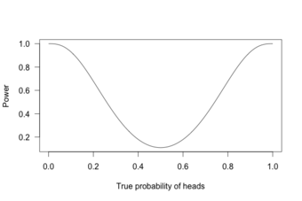
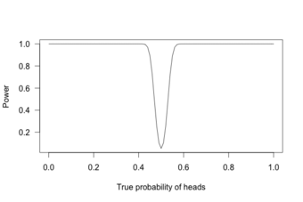
A different distribution is defined as that of the random variable defined, for a given constant
, by:
This random variable has a noncentral
-distribution with noncentrality parameter
. This distribution is important in studies of the power of Student’s
-test.
Shape
The probability density function is symmetric; its overall shape resembles the bell shape of a normally distributed variable with mean
and variance
, except that it is a bit lower and wider. In more technical terms, it has heavier tails, meaning that it is more prone to producing values that fall far from its mean. This makes it useful for understanding the statistical behavior of certain types of ratios of random quantities, in which variation in the denominator is amplified and may produce outlying values when the denominator of the ratio falls close to zero. As the number of degrees of freedom grows, the
-distribution approaches the normal distribution with mean
and variance
.
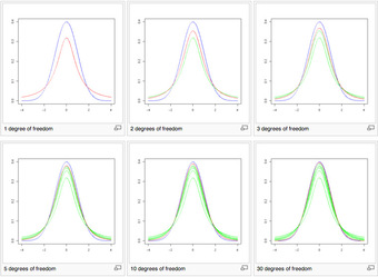
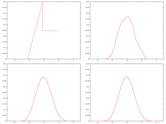
Shape of the
-Distribution
These images show the density of the
-distribution (red) for increasing values of
(1, 2, 3, 5, 10, and 30 degrees of freedom). The normal distribution is shown as a blue line for comparison. Previous plots are shown in green. Note that the
-distribution becomes closer to the normal distribution as
increases.
Uses
Student’s
-distribution arises in a variety of statistical estimation problems where the goal is to estimate an unknown parameter, such as a mean value, in a setting where the data are observed with additive errors. If (as in nearly all practical statistical work) the population standard deviation of these errors is unknown and has to be estimated from the data, the
-distribution is often used to account for the extra uncertainty that results from this estimation. In most such problems, if the standard deviation of the errors were known, a normal distribution would be used instead of the
-distribution.
Confidence intervals and hypothesis tests are two statistical procedures in which the quantiles of the sampling distribution of a particular statistic (e.g., the standard score) are required. In any situation where this statistic is a linear function of the data, divided by the usual estimate of the standard deviation, the resulting quantity can be rescaled and centered to follow Student’s
-distribution. Statistical analyses involving means, weighted means, and regression coefficients all lead to statistics having this form.
A number of statistics can be shown to have
-distributions for samples of moderate size under null hypotheses that are of interest, so that the
-distribution forms the basis for significance tests. For example, the distribution of Spearman’s rank correlation coefficient
, in the null case (zero correlation) is well approximated by the
-distribution for sample sizes above about
.
13.1.3: Assumptions
Assumptions of a
-test depend on the population being studied and on how the data are sampled.
Learning Objective
Explain the underlying assumptions of a $t$-test
Key Points
Most
-test statistics have the form
, where
and
are functions of the data.
Typically,
is designed to be sensitive to the alternative hypothesis (i.e., its magnitude tends to be larger when the alternative hypothesis is true), whereas
is a scaling parameter that allows the distribution of
to be determined.
The assumptions underlying a
-test are that:
follows a standard normal distribution under the null hypothesis, and
follows a
distribution with
degrees of freedom under the null hypothesis, where
is a positive constant.
and
are independent.
Key Terms
scaling parameter
A special kind of numerical parameter of a parametric family of probability distributions; the larger the scale parameter, the more spread out the distribution.
alternative hypothesis
a rival hypothesis to the null hypothesis, whose likelihoods are compared by a statistical hypothesis test
t-test
Any statistical hypothesis test in which the test statistic follows a Student’s $t$-distribution if the null hypothesis is supported.
Most
-test statistics have the form
, where
and
are functions of the data. Typically,
is designed to be sensitive to the alternative hypothesis (i.e., its magnitude tends to be larger when the alternative hypothesis is true), whereas
is a scaling parameter that allows the distribution of
to be determined.
As an example, in the one-sample
-test:
where
is the sample mean of the data,
is the sample size, and
is the population standard deviation of the data;
in the one-sample
-test is
, where
is the sample standard deviation.
The assumptions underlying a
-test are that:
follows a standard normal distribution under the null hypothesis.
follows a
distribution with
degrees of freedom under the null hypothesis, where
is a positive constant.
and
are independent.
In a specific type of
-test, these conditions are consequences of the population being studied, and of the way in which the data are sampled. For example, in the
-test comparing the means of two independent samples, the following assumptions should be met:
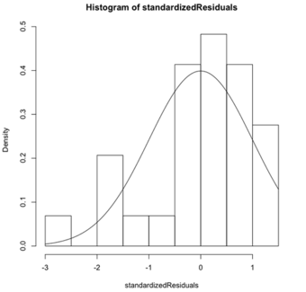
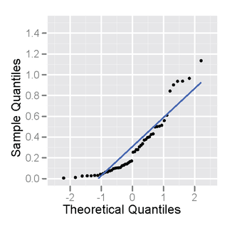
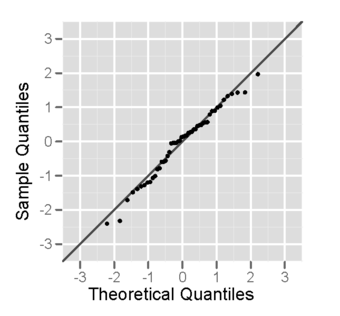
Each of the two populations being compared should follow a normal distribution. This can be tested using a normality test, or it can be assessed graphically using a normal quantile plot.
If using Student’s original definition of the
-test, the two populations being compared should have the same variance (testable using the
-test or assessable graphically using a Q-Q plot). If the sample sizes in the two groups being compared are equal, Student’s original
-test is highly robust to the presence of unequal variances. Welch’s
-test is insensitive to equality of the variances regardless of whether the sample sizes are similar.
The data used to carry out the test should be sampled independently from the two populations being compared. This is, in general, not testable from the data, but if the data are known to be dependently sampled (i.e., if they were sampled in clusters), then the classical
-tests discussed here may give misleading results.
13.1.4: t-Test for One Sample
The
-test is the most powerful parametric test for calculating the significance of a small sample mean.
Learning Objective
Derive the degrees of freedom for a t-test
Key Points
A one sample
-test has the null hypothesis, or
, of
.
The
-test is the small-sample analog of the
test, which is suitable for large samples.
For a
-test the degrees of freedom of the single mean is
because only one population parameter (the population mean) is being estimated by a sample statistic (the sample mean).
Key Terms
t-test
Any statistical hypothesis test in which the test statistic follows a Student’s $t$-distribution if the null hypothesis is supported.
degrees of freedom
any unrestricted variable in a frequency distribution
The
-test is the most powerful parametric test for calculating the significance of a small sample mean. A one sample
-test has the null hypothesis, or
, that the population mean equals the hypothesized value. Expressed formally:
where the Greek letter
represents the population mean and
represents its assumed (hypothesized) value. The
-test is the small sample analog of the
-test, which is suitable for large samples. A small sample is generally regarded as one of size
.
In order to perform a
-test, one first has to calculate the degrees of freedom. This quantity takes into account the sample size and the number of parameters that are being estimated. Here, the population parameter
is being estimated by the sample statistic
, the mean of the sample data. For a
-test the degrees of freedom of the single mean is
. This is because only one population parameter (the population mean) is being estimated by a sample statistic (the sample mean).
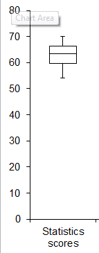
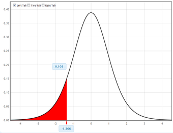
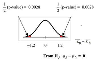
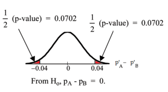
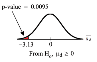
Example
A college professor wants to compare her students’ scores with the national average. She chooses a simple random sample of
students who score an average of
on a standardized test. Their scores have a standard deviation of
. The national average on the test is a
. She wants to know if her students scored significantly lower than the national average.
1. First, state the problem in terms of a distribution and identify the parameters of interest. Mention the sample. We will assume that the scores (
) of the students in the professor’s class are approximately normally distributed with unknown parameters
and
.
2. State the hypotheses in symbols and words:
i.e.: The null hypothesis is that her students scored on par with the national average.
i.e.: The alternative hypothesis is that her students scored lower than the national average.
3. Identify the appropriate test to use. Since we have a simple random sample of small size and do not know the standard deviation of the population, we will use a one-sample
-test. The formula for the
-statistic
for a one-sample test is as follows:
,
where
is the sample mean and
is the sample standard deviation. The standard deviation of the sample divided by the square root of the sample size is known as the “standard error” of the sample.
4. State the distribution of the test statistic under the null hypothesis. Under
the statistic
will follow a Student’s distribution with
degrees of freedom:
.
5. Compute the observed value
of the test statistic
, by entering the values, as follows:
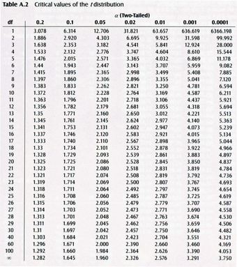
6. Determine the so-called
-value of the value
of the test statistic
. We will reject the null hypothesis for too-small values of
, so we compute the left
-value:
The Student’s distribution gives
at probabilities
and degrees of freedom
. The
-value is approximated at
.
7. Lastly, interpret the results in the context of the problem. The
-value indicates that the results almost certainly did not happen by chance and we have sufficient evidence to reject the null hypothesis. This is to say, the professor’s students did score significantly lower than the national average.
13.1.5: t-Test for Two Samples: Independent and Overlapping
Two-sample t-tests for a difference in mean involve independent samples, paired samples, and overlapping samples.
Learning Objective
Contrast paired and unpaired samples in a two-sample t-test
Key Points
For the null hypothesis, the observed t-statistic is equal to the difference between the two sample means divided by the standard error of the difference between the sample means.
The independent samples t-test is used when two separate sets of independent and identically distributed samples are obtained—one from each of the two populations being compared.
An overlapping samples t-test is used when there are paired samples with data missing in one or the other samples.
Key Terms
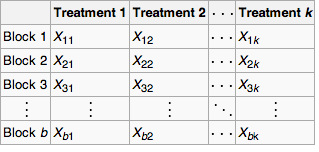
blocking
A schedule for conducting treatment combinations in an experimental study such that any effects on the experimental results due to a known change in raw materials, operators, machines, etc., become concentrated in the levels of the blocking variable.
null hypothesis
A hypothesis set up to be refuted in order to support an alternative hypothesis; presumed true until statistical evidence in the form of a hypothesis test indicates otherwise.
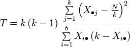
The two sample t-test is used to compare the means of two independent samples. For the null hypothesis, the observed t-statistic is equal to the difference between the two sample means divided by the standard error of the difference between the sample means. If the two population variances can be assumed equal, the standard error of the difference is estimated from the weighted variance about the means. If the variances cannot be assumed equal, then the standard error of the difference between means is taken as the square root of the sum of the individual variances divided by their sample size. In the latter case the estimated t-statistic must either be tested with modified degrees of freedom, or it can be tested against different critical values. A weighted t-test must be used if the unit of analysis comprises percentages or means based on different sample sizes.
The two-sample t-test is probably the most widely used (and misused) statistical test. Comparing means based on convenience sampling or non-random allocation is meaningless. If, for any reason, one is forced to use haphazard rather than probability sampling, then every effort must be made to minimize selection bias.
Unpaired and Overlapping Two-Sample T-Tests
Two-sample t-tests for a difference in mean involve independent samples, paired samples and overlapping samples. Paired t-tests are a form of blocking, and have greater power than unpaired tests when the paired units are similar with respect to “noise factors” that are independent of membership in the two groups being compared. In a different context, paired t-tests can be used to reduce the effects of confounding factors in an observational study.
Independent Samples
The independent samples t-test is used when two separate sets of independent and identically distributed samples are obtained, one from each of the two populations being compared. For example, suppose we are evaluating the effect of a medical treatment, and we enroll 100 subjects into our study, then randomize 50 subjects to the treatment group and 50 subjects to the control group. In this case, we have two independent samples and would use the unpaired form of the t-test .
Medical Treatment Research
Medical experimentation may utilize any two independent samples t-test.
Overlapping Samples
An overlapping samples t-test is used when there are paired samples with data missing in one or the other samples (e.g., due to selection of “I don’t know” options in questionnaires, or because respondents are randomly assigned to a subset question). These tests are widely used in commercial survey research (e.g., by polling companies) and are available in many standard crosstab software packages.
13.1.6: t-Test for Two Samples: Paired
Paired-samples
-tests typically consist of a sample of matched pairs of similar units, or one group of units that has been tested twice.
Learning Objective
Criticize the shortcomings of paired-samples $t$-tests
Key Points
A paired-difference test uses additional information about the sample that is not present in an ordinary unpaired testing situation, either to increase the statistical power or to reduce the effects of confounders.
-tests are carried out as paired difference tests for normally distributed differences where the population standard deviation of the differences is not known.
A paired samples
-test based on a “matched-pairs sample” results from an unpaired sample that is subsequently used to form a paired sample, by using additional variables that were measured along with the variable of interest.
Paired samples
-tests are often referred to as “dependent samples
-tests” (as are
-tests on overlapping samples).
Key Terms
paired difference test
A type of location test that is used when comparing two sets of measurements to assess whether their population means differ.
confounding
Describes a phenomenon in which an extraneous variable in a statistical model correlates (positively or negatively) with both the dependent variable and the independent variable; confounder = noun form.
Paired Difference Test
In statistics, a paired difference test is a type of location test used when comparing two sets of measurements to assess whether their population means differ. A paired difference test uses additional information about the sample that is not present in an ordinary unpaired testing situation, either to increase the statistical power or to reduce the effects of confounders.
-tests are carried out as paired difference tests for normally distributed differences where the population standard deviation of the differences is not known.
Paired-Samples
-Test
Paired samples
-tests typically consist of a sample of matched pairs of similar units, or one group of units that has been tested twice (a “repeated measures”
-test).
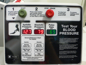
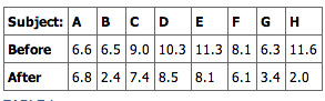
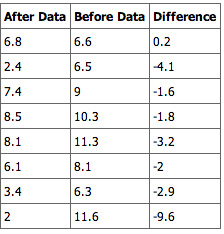
A typical example of the repeated measures t-test would be where subjects are tested prior to a treatment, say for high blood pressure, and the same subjects are tested again after treatment with a blood-pressure lowering medication . By comparing the same patient’s numbers before and after treatment, we are effectively using each patient as their own control. That way the correct rejection of the null hypothesis (here: of no difference made by the treatment) can become much more likely, with statistical power increasing simply because the random between-patient variation has now been eliminated.
Blood Pressure Treatment
A typical example of a repeated measures
-test is in the treatment of patients with high blood pressure to determine the effectiveness of a particular medication.
Note, however, that an increase of statistical power comes at a price: more tests are required, each subject having to be tested twice. Because half of the sample now depends on the other half, the paired version of Student’s
-test has only
degrees of freedom (with
being the total number of observations. Pairs become individual test units, and the sample has to be doubled to achieve the same number of degrees of freedom.
A paired-samples
-test based on a “matched-pairs sample” results from an unpaired sample that is subsequently used to form a paired sample, by using additional variables that were measured along with the variable of interest. The matching is carried out by identifying pairs of values consisting of one observation from each of the two samples, where the pair is similar in terms of other measured variables. This approach is sometimes used in observational studies to reduce or eliminate the effects of confounding factors.
Paired-samples
-tests are often referred to as “dependent samples
-tests” (as are
-tests on overlapping samples).
13.1.7: Calculations for the t-Test: One Sample
The following is a discussion on explicit expressions that can be used to carry out various
-tests.
Learning Objective
Assess a null hypothesis in a one-sample $t$-test
Key Points
In each case, the formula for a test statistic that either exactly follows or closely approximates a
-distribution under the null hypothesis is given.
Also, the appropriate degrees of freedom are given in each case.
Once a
-value is determined, a
-value can be found using a table of values from Student’s
-distribution.
If the calculated
-value is below the threshold chosen for statistical significance (usually the
, the
, or
level), then the null hypothesis is rejected in favor of the alternative hypothesis.
Key Terms
standard error
A measure of how spread out data values are around the mean, defined as the square root of the variance.
p-value
The probability of obtaining a test statistic at least as extreme as the one that was actually observed, assuming that the null hypothesis is true.
The following is a discussion on explicit expressions that can be used to carry out various
-tests. In each case, the formula for a test statistic that either exactly follows or closely approximates a
-distribution under the null hypothesis is given. Also, the appropriate degrees of freedom are given in each case. Each of these statistics can be used to carry out either a one-tailed test or a two-tailed test.
Once a
-value is determined, a
-value can be found using a table of values from Student’s
-distribution. If the calculated
-value is below the threshold chosen for statistical significance (usually the
, the
, or
level), then the null hypothesis is rejected in favor of the alternative hypothesis.
One-Sample T-Test
In testing the null hypothesis that the population mean is equal to a specified value
, one uses the statistic:
where
is the sample mean,
is the sample standard deviation of the sample and
is the sample size. The degrees of freedom used in this test is
.
Slope of a Regression
Suppose one is fitting the model:
where
are known,
and
are unknown, and
are independent identically normally distributed random errors with expected value
and unknown variance
, and
are observed. It is desired to test the null hypothesis that the slope
is equal to some specified value
(often taken to be
, in which case the hypothesis is that
and
are unrelated). Let
and
be least-squares estimators, and let
and
, respectively, be the standard errors of those least-squares estimators. Then,
has a
-distribution with
degrees of freedom if the null hypothesis is true. The standard error of the slope coefficient is:
can be written in terms of the residuals
:
Therefore, the sum of the squares of residuals, or
, is given by:
Then, the
-score is given by:
13.1.8: Calculations for the t-Test: Two Samples
The following is a discussion on explicit expressions that can be used to carry out various t-tests.
Learning Objective
Calculate the t value for different types of sample sizes and variances in an independent two-sample t-test
Key Points
A two-sample t-test for equal sample sizes and equal variances is only used when both the two sample sizes are equal and it can be assumed that the two distributions have the same variance.
A two-sample t-test for unequal sample sizes and equal variances is used only when it can be assumed that the two distributions have the same variance.
A two-sample t-test for unequal (or equal) sample sizes and unequal variances (also known as Welch’s t-test) is used only when the two population variances are assumed to be different and hence must be estimated separately.
Key Terms
pooled variance
A method for estimating variance given several different samples taken in different circumstances where the mean may vary between samples but the true variance is assumed to remain the same.
degrees of freedom
any unrestricted variable in a frequency distribution
The following is a discussion on explicit expressions that can be used to carry out various t-tests. In each case, the formula for a test statistic that either exactly follows or closely approximates a t-distribution under the null hypothesis is given. Also, the appropriate degrees of freedom are given in each case. Each of these statistics can be used to carry out either a one-tailed test or a two-tailed test.
Once a t-value is determined, a p-value can be found using a table of values from Student’s t-distribution. If the calculated p-value is below the threshold chosen for statistical significance (usually the 0.10, the 0.05, or 0.01 level), then the null hypothesis is rejected in favor of the alternative hypothesis.
Independent Two-Sample T-Test
Equal Sample Sizes, Equal Variance
This test is only used when both:
the two sample sizes (that is, the number, n, of participants of each group) are equal; and
it can be assumed that the two distributions have the same variance.
Violations of these assumptions are discussed below. The t-statistic to test whether the means are different can be calculated as follows:
,
where
.
Here,
is the grand standard deviation (or pooled standard deviation), 1 = group one, 2 = group two. The denominator of t is the standard error of the difference between two means.
For significance testing, the degrees of freedom for this test is 2n − 2 where n is the number of participants in each group.
Unequal Sample Sizes, Equal Variance
This test is used only when it can be assumed that the two distributions have the same variance. The t-statistic to test whether the means are different can be calculated as follows:
,
where .
Pooled Variance
This is the formula for a pooled variance in a two-sample t-test with unequal sample size but equal variances.
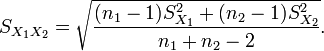
is an estimator of the common standard deviation of the two samples: it is defined in this way so that its square is an unbiased estimator of the common variance whether or not the population means are the same. In these formulae, n = number of participants, 1 = group one, 2 = group two. n − 1 is the number of degrees of freedom for either group, and the total sample size minus two (that is, n1 + n2 − 2) is the total number of degrees of freedom, which is used in significance testing.
This test, also known as Welch’s t-test, is used only when the two population variances are assumed to be different (the two sample sizes may or may not be equal) and hence must be estimated separately. The t-statistic to test whether the population means are different is calculated as:
where .
Unpooled Variance
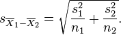
This is the formula for a pooled variance in a two-sample t-test with unequal or equal sample sizes but unequal variances.
Here s2 is the unbiased estimator of the variance of the two samples, ni = number of participants in group i, i=1 or 2. Note that in this case
is not a pooled variance. For use in significance testing, the distribution of the test statistic is approximated as an ordinary Student’s t-distribution with the degrees of freedom calculated using:
.
Welch–Satterthwaite Equation
This is the formula for calculating the degrees of freedom in Welsh’s t-test.
This is known as the Welch–Satterthwaite equation. The true distribution of the test statistic actually depends (slightly) on the two unknown population variances.
13.1.9: Multivariate Testing
Hotelling’s
-square statistic allows for the testing of hypotheses on multiple (often correlated) measures within the same sample.
Learning Objective
Summarize Hotelling’s $T$-squared statistics for one- and two-sample multivariate tests
Key Points
Hotelling’s
-squared distribution is important because it arises as the distribution of a set of statistics which are natural generalizations of the statistics underlying Student’s
-distribution.
In particular, the distribution arises in multivariate statistics in undertaking tests of the differences between the (multivariate) means of different populations, where tests for univariate problems would make use of a
-test.
For a one-sample multivariate test, the hypothesis is that the mean vector (
) is equal to a given vector (
).
For a two-sample multivariate test, the hypothesis is that the mean vectors (
and
) of two samples are equal.
Key Terms
Hotelling’s T-square statistic
A generalization of Student’s $t$-statistic that is used in multivariate hypothesis testing.
Type I error
An error occurring when the null hypothesis ($H_0$) is true, but is rejected.
A generalization of Student’s
-statistic, called Hotelling’s
-square statistic, allows for the testing of hypotheses on multiple (often correlated) measures within the same sample. For instance, a researcher might submit a number of subjects to a personality test consisting of multiple personality scales (e.g., the Minnesota Multiphasic Personality Inventory). Because measures of this type are usually highly correlated, it is not advisable to conduct separate univariate
-tests to test hypotheses, as these would neglect the covariance among measures and inflate the chance of falsely rejecting at least one hypothesis (type I error). In this case a single multivariate test is preferable for hypothesis testing. Hotelling’s
statistic follows a
distribution.
Hotelling’s
-squared distribution is important because it arises as the distribution of a set of statistics which are natural generalizations of the statistics underlying Student’s
-distribution. In particular, the distribution arises in multivariate statistics in undertaking tests of the differences between the (multivariate) means of different populations, where tests for univariate problems would make use of a
-test. It is proportional to the
-distribution.
One-sample
Test
For a one-sample multivariate test, the hypothesis is that the mean vector (
) is equal to a given vector (
). The test statistic is defined as follows:
where
is the sample size,
is the vector of column means and
is a
sample covariance matrix.
Two-Sample T2 Test
For a two-sample multivariate test, the hypothesis is that the mean vectors (
) of two samples are equal. The test statistic is defined as:
13.1.10: Alternatives to the t-Test
When the normality assumption does not hold, a nonparametric alternative to the
-test can often have better statistical power.
Learning Objective
Explain how Wilcoxon Rank Sum tests are applied to data distributions
Key Points
The
-test provides an exact test for the equality of the means of two normal populations with unknown, but equal, variances.
The Welch’s
-test is a nearly exact test for the case where the data are normal but the variances may differ.
For moderately large samples and a one-tailed test, the
is relatively robust to moderate violations of the normality assumption.
If the sample size is large, Slutsky’s theorem implies that the distribution of the sample variance has little effect on the distribution of the test statistic.
For two independent samples when the data distributions are asymmetric (that is, the distributions are skewed) or the distributions have large tails, then the Wilcoxon Rank Sum test can have three to four times higher power than the
-test.
The nonparametric counterpart to the paired-samples
-test is the Wilcoxon signed-rank test for paired samples.
Key Terms
central limit theorem
The theorem that states: If the sum of independent identically distributed random variables has a finite variance, then it will be (approximately) normally distributed.
Wilcoxon Rank Sum test
A non-parametric test of the null hypothesis that two populations are the same against an alternative hypothesis, especially that a particular population tends to have larger values than the other.
Wilcoxon signed-rank test
A nonparametric statistical hypothesis test used when comparing two related samples, matched samples, or repeated measurements on a single sample to assess whether their population mean ranks differ (i.e., it is a paired difference test).
The
-test provides an exact test for the equality of the means of two normal populations with unknown, but equal, variances. The Welch’s
-test is a nearly exact test for the case where the data are normal but the variances may differ. For moderately large samples and a one-tailed test, the
is relatively robust to moderate violations of the normality assumption.
For exactness, the
-test and
-test require normality of the sample means, and the
-test additionally requires that the sample variance follows a scaled
distribution, and that the sample mean and sample variance be statistically independent. Normality of the individual data values is not required if these conditions are met. By the central limit theorem, sample means of moderately large samples are often well-approximated by a normal distribution even if the data are not normally distributed. For non-normal data, the distribution of the sample variance may deviate substantially from a
distribution. If the data are substantially non-normal and the sample size is small, the
-test can give misleading results. However, if the sample size is large, Slutsky’s theorem implies that the distribution of the sample variance has little effect on the distribution of the test statistic.
Slutsky’s theorem extends some properties of algebraic operations on convergent sequences of real numbers to sequences of random variables. The theorem was named after Eugen Slutsky. The statement is as follows:
Let
,
be sequences of scalar/vector/matrix random elements. If
converges in distribution to a random element
, and
converges in probability to a constant
, then:
where
denotes convergence in distribution.
When the normality assumption does not hold, a nonparametric alternative to the
-test can often have better statistical power. For example, for two independent samples when the data distributions are asymmetric (that is, the distributions are skewed) or the distributions have large tails, then the Wilcoxon Rank Sum test (also known as the Mann-Whitney
test) can have three to four times higher power than the
-test. The nonparametric counterpart to the paired samples
-test is the Wilcoxon signed-rank test for paired samples.
One-way analysis of variance generalizes the two-sample
-test when the data belong to more than two groups.
13.1.11: Cohen’s d
Cohen’s
is a method of estimating effect size in a
-test based on means or distances between/among means.
Learning Objective
Justify Cohen’s $d$ as a method for estimating effect size in a $t$-test
Key Points
An effect size is a measure of the strength of a phenomenon (for example, the relationship between two variables in a statistical population) or a sample-based estimate of that quantity.
An effect size calculated from data is a descriptive statistic that conveys the estimated magnitude of a relationship without making any statement about whether the apparent relationship in the data reflects a true relationship in the population.
Cohen’s
is an example of a standardized measure of effect, which are used when the metrics of variables do not have intrinsic meaning, results from multiple studies are being combined, the studies use different scales, or when effect size is conveyed relative to the variability in the population.
As in any statistical setting, effect sizes are estimated with error, and may be biased unless the effect size estimator that is used is appropriate for the manner in which the data were sampled and the manner in which the measurements were made.
Cohen’s
is defined as the difference between two means divided by a standard deviation for the data:
.
Key Terms
Cohen’s d
A measure of effect size indicating the amount of different between two groups on a construct of interest in standard deviation units.
p-value
The probability of obtaining a test statistic at least as extreme as the one that was actually observed, assuming that the null hypothesis is true.
Cohen’s
is a method of estimating effect size in a
-test based on means or distances between/among means . An effect size is a measure of the strength of a phenomenon—for example, the relationship between two variables in a statistical population (or a sample-based estimate of that quantity). An effect size calculated from data is a descriptive statistic that conveys the estimated magnitude of a relationship without making any statement about whether the apparent relationship in the data reflects a true relationship in the population. In that way, effect sizes complement inferential statistics such as
-values. Among other uses, effect size measures play an important role in meta-analysis studies that summarize findings from a specific area of research, and in statistical power analyses.
Cohen’s
Plots of the densities of Gaussian distributions showing different Cohen’s effect sizes.
The concept of effect size already appears in everyday language. For example, a weight loss program may boast that it leads to an average weight loss of 30 pounds. In this case, 30 pounds is an indicator of the claimed effect size. Another example is that a tutoring program may claim that it raises school performance by one letter grade. This grade increase is the claimed effect size of the program. These are both examples of “absolute effect sizes,” meaning that they convey the average difference between two groups without any discussion of the variability within the groups.
Reporting effect sizes is considered good practice when presenting empirical research findings in many fields. The reporting of effect sizes facilitates the interpretation of the substantive, as opposed to the statistical, significance of a research result. Effect sizes are particularly prominent in social and medical research.
Cohen’s
is an example of a standardized measure of effect. Standardized effect size measures are typically used when the metrics of variables being studied do not have intrinsic meaning (e.g., a score on a personality test on an arbitrary scale), when results from multiple studies are being combined, when some or all of the studies use different scales, or when it is desired to convey the size of an effect relative to the variability in the population. In meta-analysis, standardized effect sizes are used as a common measure that can be calculated for different studies and then combined into an overall summary.
As in any statistical setting, effect sizes are estimated with error, and may be biased unless the effect size estimator that is used is appropriate for the manner in which the data were sampled and the manner in which the measurements were made. An example of this is publication bias, which occurs when scientists only report results when the estimated effect sizes are large or are statistically significant. As a result, if many researchers are carrying out studies under low statistical power, the reported results are biased to be stronger than true effects, if any.
Relationship to Test Statistics
Sample-based effect sizes are distinguished from test statistics used in hypothesis testing in that they estimate the strength of an apparent relationship, rather than assigning a significance level reflecting whether the relationship could be due to chance. The effect size does not determine the significance level, or vice-versa. Given a sufficiently large sample size, a statistical comparison will always show a significant difference unless the population effect size is exactly zero. For example, a sample Pearson correlation coefficient of
is strongly statistically significant if the sample size is
. Reporting only the significant
-value from this analysis could be misleading if a correlation of
is too small to be of interest in a particular application.
Cohen’s D
Cohen’s
is defined as the difference between two means divided by a standard deviation for the data:
Cohen’s
is frequently used in estimating sample sizes. A lower Cohen’s
indicates a necessity of larger sample sizes, and vice versa, as can subsequently be determined together with the additional parameters of desired significance level and statistical power.
The precise definition of the standard deviation s was not originally made explicit by Jacob Cohen; he defined it (using the symbol
) as “the standard deviation of either population” (since they are assumed equal). Other authors make the computation of the standard deviation more explicit with the following definition for a pooled standard deviation with two independent samples.
13.2: The Chi-Squared Test
13.2.1: Categorical Data and the Multinomial Experiment
The multinomial experiment is the test of the null hypothesis that the parameters of a multinomial distribution equal specified values.
Learning Objective
Explain the multinomial experiment for testing a null hypothesis
Key Points
The multinomial experiment is really an extension of the binomial experiment, in which there were only two categories: success or failure.
The multinomial experiment consists of
identical and independent trials with
possible outcomes for each trial.
For n independent trials each of which leads to a success for exactly one of
categories, with each category having a given fixed success probability, the multinomial distribution gives the probability of any particular combination of numbers of successes for the various categories.
Key Terms
binomial distribution
the discrete probability distribution of the number of successes in a sequence of $n$ independent yes/no experiments, each of which yields success with probability $p$
multinomial distribution
A generalization of the binomial distribution; gives the probability of any particular combination of numbers of successes for the various categories.
The Multinomial Distribution
In probability theory, the multinomial distribution is a generalization of the binomial distribution. For
independent trials, each of which leads to a success for exactly one of
categories and with each category having a given fixed success probability, the multinomial distribution gives the probability of any particular combination of numbers of successes for the various categories.
The binomial distribution is the probability distribution of the number of successes for one of just two categories in
independent Bernoulli trials, with the same probability of success on each trial. In a multinomial distribution, the analog of the Bernoulli distribution is the categorical distribution, where each trial results in exactly one of some fixed finite number
of possible outcomes, with probabilities
(so that
for
and the sum is
), and there are
independent trials. Then if the random variables Xi indicate the number of times outcome number
is observed over the
trials, the vector
follows a multinomial distribution with parameters
and
, where
.
The Multinomial Experiment
In statistics, the multinomial experiment is the test of the null hypothesis that the parameters of a multinomial distribution equal specified values. It is used for categorical data. It is really an extension of the binomial experiment, where there were only two categories: success or failure. One example of a multinomial experiment is asking which of six candidates a voter preferred in an election.
Properties for the Multinomial Experiment
The experiment consists of
identical trials.
There are
possible outcomes for each trial. These outcomes are sometimes called classes, categories, or cells.
The probabilities of the
outcomes, denoted by
,
,
,
, remain the same from trial to trial, and they sum to one.
The trials are independent.
The random variables of interest are the cell counts
,
,
,
, which refer to the number of observations that fall into each of the
categories.
13.2.2: Structure of the Chi-Squared Test
The chi-square test is used to determine if a distribution of observed frequencies differs from the theoretical expected frequencies.
Learning Objective
Apply the chi-square test to approximate the probability of an event, distinguishing the different sample conditions in which it can be applied
Key Points
A chi-square test statistic is a measure of how different the data we observe are to what we would expect to observe if the variables were truly independent.
The higher the test-statistic, the more likely that the data we observe did not come from independent variables.
The chi-square distribution shows us how likely it is that the test statistic value was due to chance.
If the difference between what we observe and what we expect from independent variables is large (and not just by chance), then we reject the null hypothesis that the two variables are independent and conclude that there is a relationship between the variables.
Two types of chi-square tests include the test for goodness of fit and the test for independence.
Certain assumptions must be made when conducting a goodness of fit test, including a simple random sample, a large enough sample size, independence, and adequate expected cell count.
Key Terms
degrees of freedom
any unrestricted variable in a frequency distribution
Fisher’s exact test
a statistical significance test used in the analysis of contingency tables, in which the significance of the deviation from a null hypothesis can be calculated exactly, rather than relying on an approximation that becomes exact in the limit as the sample size grows to infinity
The chi-square (
) test is a nonparametric statistical technique used to determine if a distribution of observed frequencies differs from the theoretical expected frequencies. Chi-square statistics use nominal (categorical) or ordinal level data. Thus, instead of using means and variances, this test uses frequencies.
Generally, the chi-squared statistic summarizes the discrepancies between the expected number of times each outcome occurs (assuming that the model is true) and the observed number of times each outcome occurs, by summing the squares of the discrepancies, normalized by the expected numbers, over all the categories.
Data used in a chi-square analysis has to satisfy the following conditions:
Simple random sample – The sample data is a random sampling from a fixed distribution or population where each member of the population has an equal probability of selection. Variants of the test have been developed for complex samples, such as where the data is weighted.
Sample size (whole table) – A sample with a sufficiently large size is assumed. If a chi squared test is conducted on a sample with a smaller size, then the chi squared test will yield an inaccurate inference. The researcher, by using chi squared test on small samples, might end up committing a Type II error.
Expected cell count – Adequate expected cell counts. Some require 5 or more, and others require 10 or more. A common rule is 5 or more in all cells of a 2-by-2 table, and 5 or more in 80% of cells in larger tables, but no cells with zero expected count.
Independence – The observations are always assumed to be independent of each other. This means chi-squared cannot be used to test correlated data (like matched pairs or panel data).
There are two types of chi-square test:
The Chi-square test for goodness of fit, which compares the expected and observed values to determine how well an experimenter’s predictions fit the data.
The Chi-square test for independence, which compares two sets of categories to determine whether the two groups are distributed differently among the categories.
How Do We Perform a Chi-Square Test?
First, we calculate a chi-square test statistic. The higher the test-statistic, the more likely that the data we observe did not come from independent variables.
Second, we use the chi-square distribution. We may observe data that give us a high test-statistic just by chance, but the chi-square distribution shows us how likely it is. The chi-square distribution takes slightly different shapes depending on how many categories (degrees of freedom) our variables have. Interestingly, when the degrees of freedom get very large, the shape begins to look like the bell curve we know and love. This is a property shared by the
-distribution.
If the difference between what we observe and what we expect from independent variables is large (that is, the chi-square distribution tells us it is unlikely to be that large just by chance) then we reject the null hypothesis that the two variables are independent. Instead, we favor the alternative that there is a relationship between the variables. Therefore, chi-square can help us discover that there is a relationship but cannot look too deeply into what that relationship is.
Problems
The approximation to the chi-squared distribution breaks down if expected frequencies are too low. It will normally be acceptable so long as no more than 20% of the events have expected frequencies below 5. Where there is only 1 degree of freedom, the approximation is not reliable if expected frequencies are below 10. In this case, a better approximation can be obtained by reducing the absolute value of each difference between observed and expected frequencies by 0.5 before squaring. This is called Yates’s correction for continuity.
In cases where the expected value,
, is found to be small (indicating a small underlying population probability, and/or a small number of observations), the normal approximation of the multinomial distribution can fail. In such cases it is found to be more appropriate to use the
-test, a likelihood ratio-based test statistic. Where the total sample size is small, it is necessary to use an appropriate exact test, typically either the binomial test or (for contingency tables) Fisher’s exact test. However, note that this test assumes fixed and known totals in all margins, an assumption which is typically false.
13.2.3: How Fisher Used the Chi-Squared Test
Fisher’s exact test is preferable to a chi-square test when sample sizes are small, or the data are very unequally distributed.
Learning Objective
Calculate statistical significance by employing Fisher’s exact test
Key Points
Fisher’s exact test is a statistical significance test used in the analysis of contingency tables.
Fisher’s exact test is useful for categorical data that result from classifying objects in two different ways.
It is used to examine the significance of the association (contingency) between the two kinds of classification.
The usual rule of thumb for deciding whether the chi-squared approximation is good enough is that the chi-squared test is not suitable when the expected values in any of the cells of a contingency table are below 5, or below 10 when there is only one degree of freedom.
Fisher’s exact test becomes difficult to calculate with large samples or well-balanced tables, but fortunately these are exactly the conditions where the chi-squared test is appropriate.
Key Terms
p-value
The probability of obtaining a test statistic at least as extreme as the one that was actually observed, assuming that the null hypothesis is true.
hypergeometric distribution
a discrete probability distribution that describes the number of successes in a sequence of $n$ draws from a finite population without replacement
contingency table
a table presenting the joint distribution of two categorical variables
Fisher’s exact test is a statistical significance test used in the analysis of contingency tables. Although in practice it is employed when sample sizes are small, it is valid for all sample sizes. It is named after its inventor, R. A. Fisher. Fisher’s exact test is one of a class of exact tests, so called because the significance of the deviation from a null hypothesis can be calculated exactly, rather than relying on an approximation that becomes exact in the limit as the sample size grows to infinity. Fisher is said to have devised the test following a comment from Dr. Muriel Bristol, who claimed to be able to detect whether the tea or the milk was added first to her cup.
Sir Ronald Fisher
Sir Ronald Fisher is the namesake for Fisher’s exact test.
Purpose and Scope
The test is useful for categorical data that result from classifying objects in two different ways. It is used to examine the significance of the association (contingency) between the two kinds of classification. In Fisher’s original example, one criterion of classification could be whether milk or tea was put in the cup first, and the other could be whether Dr. Bristol thinks that the milk or tea was put in first. We want to know whether these two classifications are associated—that is, whether Dr. Bristol really can tell whether milk or tea was poured in first. Most uses of the Fisher test involve, like this example, a
contingency table. The
-value from the test is computed as if the margins of the table are fixed (i.e., as if, in the tea-tasting example, Dr. Bristol knows the number of cups with each treatment [milk or tea first] and will, therefore, provide guesses with the correct number in each category). As pointed out by Fisher, under a null hypothesis of independence, this leads to a hypergeometric distribution of the numbers in the cells of the table.
With large samples, a chi-squared test can be used in this situation. However, the significance value it provides is only an approximation, because the sampling distribution of the test statistic that is calculated is only approximately equal to the theoretical chi-squared distribution. The approximation is inadequate when sample sizes are small, or the data are very unequally distributed among the cells of the table, resulting in the cell counts predicted on the null hypothesis (the “expected values”) being low. The usual rule of thumb for deciding whether the chi-squared approximation is good enough is that the chi-squared test is not suitable when the expected values in any of the cells of a contingency table are below 5, or below 10 when there is only one degree of freedom. In fact, for small, sparse, or unbalanced data, the exact and asymptotic
-values can be quite different and may lead to opposite conclusions concerning the hypothesis of interest. In contrast, the Fisher test is, as its name states, exact as long as the experimental procedure keeps the row and column totals fixed. Therefore, it can be used regardless of the sample characteristics. It becomes difficult to calculate with large samples or well-balanced tables, but fortunately these are exactly the conditions where the chi-squared test is appropriate.
For hand calculations, the test is only feasible in the case of a
contingency table. However, the principle of the test can be extended to the general case of an
table, and some statistical packages provide a calculation for the more general case.
13.2.4: Goodness of Fit
The goodness of fit test determines whether the data “fit” a particular distribution or not.
Learning Objective
Outline the procedure for the goodness of fit test
Key Points
The test statistic for a goodness-of-fit test is:
, where
is the observed values (data),
is the expected values (from theory), and
is the number of different data cells or categories.
The goodness-of-fit test is almost always right tailed. If the observed values and the corresponding expected values are not close to each other, then the test statistic can get very large and will be way out in the right tail of the chi-square curve.
If the observed values and the corresponding expected values are not close to each other, then the test statistic can get very large and will be way out in the right tail of the chi-square curve.
The null hypothesis for a chi-square test is that the observed values are close to the predicted values.
The alternative hypothesis is that they are not close to the predicted values.
Key Terms
binomial distribution
the discrete probability distribution of the number of successes in a sequence of n independent yes/no experiments, each of which yields success with probability $p$
goodness of fit
how well a statistical model fits a set of observations
Procedure for the Goodness of Fit Test
Goodness of fit means how well a statistical model fits a set of observations. A measure of goodness of fit typically summarize the discrepancy between observed values and the values expected under the model in question. Such measures can be used in statistical hypothesis testing, e.g., to test for normality of residuals or to test whether two samples are drawn from identical distributions.
In this type of hypothesis test, we determine whether the data “fit” a particular distribution or not. For example, we may suspect that our unknown data fits a binomial distribution. We use a chi-square test (meaning the distribution for the hypothesis test is chi-square) to determine if there is a fit or not. The null and the alternate hypotheses for this test may be written in sentences or may be stated as equations or inequalities.
The test statistic for a goodness-of-fit test is:
where
is the observed values (data),
is the expected values (from theory), and
is the number of different data cells or categories.
The observed values are the data values and the expected values are the values we would expect to get if the null hypothesis was true. The degrees of freedom are found as follows:
where
is the number of categories.The goodness-of-fit test is almost always right tailed. If the observed values and the corresponding expected values are not close to each other, then the test statistic can get very large and will be way out in the right tail of the chi-square curve.
As an example, suppose a coin is tossed 100 times. The outcomes would be expected to be 50 heads and 50 tails. If 47 heads and 53 tails are observed instead, does this deviation occur because the coin is biased, or is it by chance?
The null hypothesis for the above experiment is that the observed values are close to the predicted values. The alternative hypothesis is that they are not close to the predicted values. These hypotheses hold for all chi-square goodness of fit tests. Thus in this case the null and alternative hypotheses corresponds to:
Null hypothesis: The coin is fair.
Alternative hypothesis: The coin is biased.
We calculate chi-square by substituting values for
and
.
For heads:
For tails:
The sum of these categories is:
Significance of the chi-square test for goodness of fit value is established by calculating the degree of freedom
(the Greek letter nu) and by using the chi-square distribution table. The
in a chi-square goodness of fit test is equal to the number of categories,
, minus one (
). This is done in order to check if the null hypothesis is valid or not, by looking at the critical chi-square value from the table that corresponds to the calculated
. If the calculated chi-square is greater than the value in the table, then the null hypothesis is rejected, and it is concluded that the predictions made were incorrect. In the above experiment,
. The critical value for a chi-square for this example at
and
is
, which is greater than
. Therefore the null hypothesis is not rejected, and the coin toss was fair.
Chi-Square Distribution
Plot of the chi-square distribution for values of
.
13.2.5: Inferences of Correlation and Regression
The chi-square test of association allows us to evaluate associations (or correlations) between categorical data.
Learning Objective
Calculate the adjusted standardized residuals for a chi-square test
Key Points
The chi-square test indicates whether there is an association between two categorical variables, but unlike the correlation coefficient between two quantitative variables, it does not in itself give an indication of the strength of the association.
In order to describe the association more fully, it is necessary to identify the cells that have large differences between the observed and expected frequencies. These differences are referred to as residuals, and they can be standardized and adjusted to follow a Normal distribution.
The larger the absolute value of the residual, the larger the difference between the observed and expected frequencies, and therefore the more significant the association between the two variables.
Key Terms
correlation coefficient
Any of the several measures indicating the strength and direction of a linear relationship between two random variables.
residuals
The difference between the observed value and the estimated function value.
The chi-square test of association allows us to evaluate associations (or correlations) between categorical data. It indicates whether there is an association between two categorical variables, but unlike the correlation coefficient between two quantitative variables, it does not in itself give an indication of the strength of the association.
In order to describe the association more fully, it is necessary to identify the cells that have large differences between the observed and expected frequencies. These differences are referred to as residuals, and they can be standardized and adjusted to follow a normal distribution with mean
and standard deviation
. The adjusted standardized residuals,
, are given by:
where
is the total frequency for row
,
is the total frequency for column
, and
is the overall total frequency. The larger the absolute value of the residual, the larger the difference between the observed and expected frequencies, and therefore the more significant the association between the two variables.
Table 1
Numbers of patients classified by site of central venous cannula and infectious complication. This table shows the proportions of patients in the sample with cannulae sited at the internal jugular, subclavian and femoral veins. Using the above formula to find the adjusted standardized residual for those with cannulae sited at the internal jugular and no infectious complications yields:
. Subclavian site/no infectious complication has the largest residual at 6.2. Because it is positive, there are more individuals than expected with no infectious complications where the subclavian central line site was used. As these residuals follow a Normal distribution with mean 0 and standard deviation 1, all absolute values over 2 are significant. The association between femoral site/no infectious complication is also significant, but because the residual is negative, there are fewer individuals than expected in this cell. When the subclavian central line site was used, infectious complications appear to be less likely than when the other two sites were used.
Table 2
The adjusted standardized residuals from Table 1.
13.2.6: Example: Test for Goodness of Fit
The Chi-square test for goodness of fit compares the expected and observed values to determine how well an experimenter’s predictions fit the data.
Learning Objective
Support the use of Pearson’s chi-squared test to measure goodness of fit
Key Points
Pearson’s chi-squared test uses a measure of goodness of fit, which is the sum of differences between observed and expected outcome frequencies, each squared and divided by the expectation.
If the value of the chi-square test statistic is greater than the value in the chi-square table, then the null hypothesis is rejected.
In this text, we examine a goodness of fit test as follows: for a population of employees, do the days for the highest number of absences occur with equal frequencies during a five day work week?
Key Term
null hypothesis
A hypothesis set up to be refuted in order to support an alternative hypothesis; presumed true until statistical evidence in the form of a hypothesis test indicates otherwise.
Pearson’s chi-squared test uses a measure of goodness of fit, which is the sum of differences between observed and expected outcome frequencies (that is, counts of observations), each squared and divided by the expectation:
where
is an observed frequency (i.e. count) for bin
and
= an expected (theoretical) frequency for bin
, asserted by the null hypothesis.
The expected frequency is calculated by:
where
is the cumulative distribution function for the distribution being tested,
is the upper limit for class
,
is the lower limit for class
, and
is the sample size.
Example
Employers want to know which days of the week employees are absent in a five day work week. Most employers would like to believe that employees are absent equally during the week. Suppose a random sample of 60 managers were asked on which day of the week did they have the highest number of employee absences. The results were distributed as follows:
Monday: 15
Tuesday: 12
Wednesday: 9
Thursday: 9
Friday: 15
Solution
The null and alternate hypotheses are:
: The absent days occur with equal frequencies—that is, they fit a uniform distribution.
: The absent days occur with unequal frequencies—that is, they do not fit a uniform distribution.
If the absent days occur with equal frequencies then, out of
absent days (the total in the sample:
), there would be
absences on Monday,
on Tuesday,
on Wednesday,
on Thursday, and
on Friday. These numbers are the expected (
) values. The values in the table are the observed (
) values or data.
Calculate the
test statistic. Make a chart with the following column headings and fill in the cells:
Expected (
) values (
,
,
,
,
)
Observed (
) values (
,
,
,
,
)
Now add (sum) the values of the last column. Verify that this sum is
. This is the
test statistic.
To find the
-value, calculate
(
). This test is right-tailed. (
)
The degrees of freedom are one fewer than the number of cells:
.
Conclusion
The decision is to not reject the null hypothesis. At a
level of significance, from the sample data, there is not sufficient evidence to conclude that the absent days do not occur with equal frequencies.
13.2.7: Example: Test for Independence
The chi-square test for independence is used to determine the relationship between two variables of a sample.
Learning Objective
Explain how to calculate chi-square test for independence
Key Points
As with the goodness of fit example in the previous section, the key idea of the chi-square test for independence is a comparison of observed and expected values.
It is important to keep in mind that the chi-square test for independence only tests whether two variables are independent or not, it cannot address questions of which is greater or less.
In the example presented in this text, we examine whether boys or girls get into trouble more often in school.
The null hypothesis is that the likelihood of getting in trouble is the same for boys and girls.
We calculate a chi-square statistic of
and find a
-value of
. Therefore, we fail to reject the null hypothesis.
Key Terms
null hypothesis
A hypothesis set up to be refuted in order to support an alternative hypothesis; presumed true until statistical evidence in the form of a hypothesis test indicates otherwise.
alternative hypothesis
a rival hypothesis to the null hypothesis, whose likelihoods are compared by a statistical hypothesis test
The chi-square test for independence is used to determine the relationship between two variables of a sample. In this context, independence means that the two factors are not related. Typically in social science research, researchers are interested in finding factors which are related (e.g., education and income, occupation and prestige, age and voting behavior).
Suppose we want to know whether boys or girls get into trouble more often in school. Below is the table documenting the frequency of boys and girls who got into trouble in school.
Test for Independence
For our example, this table shows the tabulated results of the observed and expected frequencies.
To examine statistically whether boys got in trouble more often in school, we need to establish hypotheses for the question. The null hypothesis is that the two variables are independent. In this particular case, it is that the likelihood of getting in trouble is the same for boys and girls. The alternative hypothesis to be tested is that the likelihood of getting in trouble is not the same for boys and girls.
It is important to keep in mind that the chi-square test for independence only tests whether two variables are independent or not. It cannot address questions of which is greater or less. Using the chi-square test for independence, who gets into more trouble between boys and girls cannot be evaluated directly from the hypothesis.
As with the goodness of fit example seen previously, the key idea of the chi-square test for independence is a comparison of observed and expected values. In the case of tabular data, however, we usually do not know what the distribution should look like (as we did with tossing the coin). Rather, expected values are calculated based on the row and column totals from the table using the following equation:
expected value = (row total x column total) / total for table.
where
is the sum over that row,
is the sum over that column, and
is the sum over the entire table. The expected values (in parentheses, italics and bold) for each cell are also presented in the table above.
With the values in the table, the chi-square statistic can be calculated as follows:
In the chi-square test for independence, the degrees of freedom are found as follows:
where
is the number of rows in the table and
is the number of columns in the table. Substituting in the proper values yields:
Finally, the value calculated from the formula above is compared with values in the chi-square distribution table. The value returned from the table is
(
). Therefore, the null hypothesis is not rejected. Hence, boys are not significantly more likely to get in trouble in school than girls.
13.3: Tests for Ranked Data
13.3.1: When to Use These Tests
“Ranking” refers to the data transformation in which numerical or ordinal values are replaced by their rank when the data are sorted.
Learning Objective
Indicate why and how data transformation is performed and how this relates to ranked data.
Key Points
Data transforms are usually applied so that the data appear to more closely meet the assumptions of a statistical inference procedure that is to be applied, or to improve the interpretability or appearance of graphs.
Guidance for how data should be transformed, or whether a transform should be applied at all, should come from the particular statistical analysis to be performed.
When there is evidence of substantial skew in the data, it is common to transform the data to a symmetric distribution before constructing a confidence interval.
Data can also be transformed to make it easier to visualize them.
A final reason that data can be transformed is to improve interpretability, even if no formal statistical analysis or visualization is to be performed.
Key Terms
central limit theorem
The theorem that states: If the sum of independent identically distributed random variables has a finite variance, then it will be (approximately) normally distributed.
confidence interval
A type of interval estimate of a population parameter used to indicate the reliability of an estimate.
data transformation
The application of a deterministic mathematical function to each point in a data set.
In statistics, “ranking” refers to the data transformation in which numerical or ordinal values are replaced by their rank when the data are sorted. If, for example, the numerical data 3.4, 5.1, 2.6, 7.3 are observed, the ranks of these data items would be 2, 3, 1 and 4 respectively. In another example, the ordinal data hot, cold, warm would be replaced by 3, 1, 2. In these examples, the ranks are assigned to values in ascending order. (In some other cases, descending ranks are used. ) Ranks are related to the indexed list of order statistics, which consists of the original dataset rearranged into ascending order.
Some kinds of statistical tests employ calculations based on ranks. Examples include:
Friedman test
Kruskal-Wallis test
Rank products
Spearman’s rank correlation coefficient
Wilcoxon rank-sum test
Wilcoxon signed-rank test
Some ranks can have non-integer values for tied data values. For example, when there is an even number of copies of the same data value, the above described fractional statistical rank of the tied data ends in
.
Data Transformation
Data transformation refers to the application of a deterministic mathematical function to each point in a data set—that is, each data point
is replaced with the transformed value
, where
is a function. Transforms are usually applied so that the data appear to more closely meet the assumptions of a statistical inference procedure that is to be applied, or to improve the interpretability or appearance of graphs.
Nearly always, the function that is used to transform the data is invertible and, generally, is continuous. The transformation is usually applied to a collection of comparable measurements. For example, if we are working with data on peoples’ incomes in some currency unit, it would be common to transform each person’s income value by the logarithm function.
Reasons for Transforming Data
Guidance for how data should be transformed, or whether a transform should be applied at all, should come from the particular statistical analysis to be performed. For example, a simple way to construct an approximate 95% confidence interval for the population mean is to take the sample mean plus or minus two standard error units. However, the constant factor 2 used here is particular to the normal distribution and is only applicable if the sample mean varies approximately normally. The central limit theorem states that in many situations, the sample mean does vary normally if the sample size is reasonably large.
However, if the population is substantially skewed and the sample size is at most moderate, the approximation provided by the central limit theorem can be poor, and the resulting confidence interval will likely have the wrong coverage probability. Thus, when there is evidence of substantial skew in the data, it is common to transform the data to a symmetric distribution before constructing a confidence interval. If desired, the confidence interval can then be transformed back to the original scale using the inverse of the transformation that was applied to the data.
Data can also be transformed to make it easier to visualize them. For example, suppose we have a scatterplot in which the points are the countries of the world, and the data values being plotted are the land area and population of each country. If the plot is made using untransformed data (e.g., square kilometers for area and the number of people for population), most of the countries would be plotted in tight cluster of points in the lower left corner of the graph. The few countries with very large areas and/or populations would be spread thinly around most of the graph’s area. Simply rescaling units (e.g., to thousand square kilometers, or to millions of people) will not change this. However, following logarithmic transformations of both area and population, the points will be spread more uniformly in the graph .
Population Versus Area Scatterplots
A scatterplot in which the areas of the sovereign states and dependent territories in the world are plotted on the vertical axis against their populations on the horizontal axis. The upper plot uses raw data. In the lower plot, both the area and population data have been transformed using the logarithm function.
A final reason that data can be transformed is to improve interpretability, even if no formal statistical analysis or visualization is to be performed. For example, suppose we are comparing cars in terms of their fuel economy. These data are usually presented as “kilometers per liter” or “miles per gallon. ” However, if the goal is to assess how much additional fuel a person would use in one year when driving one car compared to another, it is more natural to work with the data transformed by the reciprocal function, yielding liters per kilometer, or gallons per mile.
13.3.2: Mann-Whitney U-Test
The Mann–Whitney
-test is a non-parametric test of the null hypothesis that two populations are the same against an alternative hypothesis.
Learning Objective
Compare the Mann-Whitney $U$-test to Student’s $t$-test
Key Points
Mann-Whitney has greater efficiency than the
-test on non-normal distributions, such as a mixture of normal distributions, and it is nearly as efficient as the
-test on normal distributions.
The test involves the calculation of a statistic, usually called
, whose distribution under the null hypothesis is known.
The first method to calculate
involves choosing the sample which has the smaller ranks, then counting the number of ranks in the other sample that are smaller than the ranks in the first, then summing these counts.
The second method involves adding up the ranks for the observations which came from sample 1. The sum of ranks in sample 2 is now determinate, since the sum of all the ranks equals
, where
is the total number of observations.
Key Terms
ordinal data
A statistical data type consisting of numerical scores that exist on an ordinal scale, i.e. an arbitrary numerical scale where the exact numerical quantity of a particular value has no significance beyond its ability to establish a ranking over a set of data points.
tie
One or more equal values or sets of equal values in the data set.
The Mann–Whitney
-test is a non-parametric test of the null hypothesis that two populations are the same against an alternative hypothesis, especially that a particular population tends to have larger values than the other. It has greater efficiency than the
-test on non-normal distributions, such as a mixture of normal distributions, and it is nearly as efficient as the
-test on normal distributions.
Assumptions and Formal Statement of Hypotheses
Although Mann and Whitney developed the test under the assumption of continuous responses with the alternative hypothesis being that one distribution is stochastically greater than the other, there are many other ways to formulate the null and alternative hypotheses such that the test will give a valid test. A very general formulation is to assume that:
All the observations from both groups are independent of each other.
The responses are ordinal (i.e., one can at least say of any two observations which is the greater).
The distributions of both groups are equal under the null hypothesis, so that the probability of an observation from one population (
) exceeding an observation from the second population (
) equals the probability of an observation from
exceeding an observation from
. That is, there is a symmetry between populations with respect to probability of random drawing of a larger observation.
Under the alternative hypothesis, the probability of an observation from one population (
) exceeding an observation from the second population (
) (after exclusion of ties) is not equal to
. The alternative may also be stated in terms of a one-sided test, for example:
.
Calculations
The test involves the calculation of a statistic, usually called
, whose distribution under the null hypothesis is known. In the case of small samples, the distribution is tabulated, but for sample sizes above about 20, approximation using the normal distribution is fairly good.
There are two ways of calculating
by hand. For either method, we must first arrange all the observations into a single ranked series. That is, rank all the observations without regard to which sample they are in.
Method One
For small samples a direct method is recommended. It is very quick, and gives an insight into the meaning of the
statistic.
Choose the sample for which the ranks seem to be smaller (the only reason to do this is to make computation easier). Call this “sample 1,” and call the other sample “sample 2. “
For each observation in sample 1, count the number of observations in sample 2 that have a smaller rank (count a half for any that are equal to it). The sum of these counts is
.
Method Two
For larger samples, a formula can be used.
First, add up the ranks for the observations that came from sample 1. The sum of ranks in sample 2 is now determinate, since the sum of all the ranks equals:
where
is the total number of observations.
is then given by:
where
is the sample size for sample 1, and
is the sum of the ranks in sample 1. Note that it doesn’t matter which of the two samples is considered sample 1. The smaller value of
and
is the one used when consulting significance tables.
Example of Statement Results
In reporting the results of a Mann–Whitney test, it is important to state:
a measure of the central tendencies of the two groups (means or medians; since the Mann–Whitney is an ordinal test, medians are usually recommended)
the value of
the sample sizes
the significance level
In practice some of this information may already have been supplied and common sense should be used in deciding whether to repeat it. A typical report might run:
“Median latencies in groups
and
were
and
ms; the distributions in the two groups differed significantly (Mann–Whitney
,
,
).”
Comparison to Student’s
-Test
The
-test is more widely applicable than independent samples Student’s
-test, and the question arises of which should be preferred.
Ordinal Data
remains the logical choice when the data are ordinal but not interval scaled, so that the spacing between adjacent values cannot be assumed to be constant.
Robustness
As it compares the sums of ranks, the Mann–Whitney test is less likely than the
-test to spuriously indicate significance because of the presence of outliers (i.e., Mann–Whitney is more robust).
Efficiency
For distributions sufficiently far from normal and for sufficiently large sample sizes, the Mann-Whitney Test is considerably more efficient than the
. Overall, the robustness makes Mann-Whitney more widely applicable than the
-test. For large samples from the normal distribution, the efficiency loss compared to the
-test is only 5%, so one can recommend Mann-Whitney as the default test for comparing interval or ordinal measurements with similar distributions.
13.3.3: Wilcoxon t-Test
The Wilcoxon
-test assesses whether population mean ranks differ for two related samples, matched samples, or repeated measurements on a single sample.
Learning Objective
Break down the procedure for the Wilcoxon signed-rank t-test.
Key Points
The Wilcoxon
-test can be used as an alternative to the paired Student’s
-test,
-test for matched pairs, or the
-test for dependent samples when the population cannot be assumed to be normally distributed.
The test is named for Frank Wilcoxon who (in a single paper) proposed both the rank
-test and the rank-sum test for two independent samples.
The test assumes that data are paired and come from the same population, each pair is chosen randomly and independent and the data are measured at least on an ordinal scale, but need not be normal.
Key Terms
Wilcoxon t-test
A non-parametric statistical hypothesis test used when comparing two related samples, matched samples, or repeated measurements on a single sample to assess whether their population mean ranks differ (i.e., it is a paired-difference test).
tie
One or more equal values or sets of equal values in the data set.
The Wilcoxon signed-rank t-test is a non-parametric statistical hypothesis test used when comparing two related samples, matched samples, or repeated measurements on a single sample to assess whether their population mean ranks differ (i.e., it is a paired difference test). It can be used as an alternative to the paired Student’s
-test,
-test for matched pairs, or the
-test for dependent samples when the population cannot be assumed to be normally distributed.
The test is named for Frank Wilcoxon who (in a single paper) proposed both the rank
-test and the rank-sum test for two independent samples. The test was popularized by Siegel in his influential text book on non-parametric statistics. Siegel used the symbol
for the value defined below as
. In consequence, the test is sometimes referred to as the Wilcoxon
-test, and the test statistic is reported as a value of
. Other names may include the “
-test for matched pairs” or the “
-test for dependent samples.”
Assumptions
Data are paired and come from the same population.
Each pair is chosen randomly and independent.
The data are measured at least on an ordinal scale, but need not be normal.
Test Procedure
Let
be the sample size, the number of pairs. Thus, there are a total of
data points. For
, let
and
denote the measurements.
: The median difference between the pairs is zero.
: The median difference is not zero.
1. For
, calculate
and
, where
is the sign function.
2. Exclude pairs with
. Let
be the reduced sample size.
3. Order the remaining pairs from smallest absolute difference to largest absolute difference,
.
4. Rank the pairs, starting with the smallest as 1. Ties receive a rank equal to the average of the ranks they span. Let
denote the rank.
5. Calculate the test statistic
, the absolute value of the sum of the signed ranks:
6. As
increases, the sampling distribution of
converges to a normal distribution. Thus, for
, a
-score can be calculated as follows:
where
If
then reject
.
For
,
is compared to a critical value from a reference table. If
then reject
.
Alternatively, a
-value can be calculated from enumeration of all possible combinations of
given
.
13.3.4: Kruskal-Wallis H-Test
The Kruskal–Wallis one-way analysis of variance by ranks is a non-parametric method for testing whether samples originate from the same distribution.
Learning Objective
Summarize the Kruskal-Wallis one-way analysis of variance and outline its methodology
Key Points
The Kruskal-Wallis test is used for comparing more than two samples that are independent, or not related.
When the Kruskal-Wallis test leads to significant results, then at least one of the samples is different from the other samples.
The test does not identify where the differences occur or how many differences actually occur.
Since it is a non-parametric method, the Kruskal–Wallis test does not assume a normal distribution, unlike the analogous one-way analysis of variance.
The test does assume an identically shaped and scaled distribution for each group, except for any difference in medians.
Kruskal–Wallis is also used when the examined groups are of unequal size (different number of participants).
Key Terms
Kruskal-Wallis test
A non-parametric method for testing whether samples originate from the same distribution.
Type I error
An error occurring when the null hypothesis ($H_0$) is true, but is rejected.
chi-squared distribution
A distribution with $k$ degrees of freedom is the distribution of a sum of the squares of $k$ independent standard normal random variables.
The Kruskal–Wallis one-way analysis of variance by ranks (named after William Kruskal and W. Allen Wallis) is a non-parametric method for testing whether samples originate from the same distribution. It is used for comparing more than two samples that are independent, or not related. The parametric equivalent of the Kruskal-Wallis test is the one-way analysis of variance (ANOVA). When the Kruskal-Wallis test leads to significant results, then at least one of the samples is different from the other samples. The test does not identify where the differences occur, nor how many differences actually occur. It is an extension of the Mann–Whitney
test to 3 or more groups. The Mann-Whitney would help analyze the specific sample pairs for significant differences.
Since it is a non-parametric method, the Kruskal–Wallis test does not assume a normal distribution, unlike the analogous one-way analysis of variance. However, the test does assume an identically shaped and scaled distribution for each group, except for any difference in medians.
Kruskal–Wallis is also used when the examined groups are of unequal size (different number of participants).
Method
1. Rank all data from all groups together; i.e., rank the data from
to
ignoring group membership. Assign any tied values the average of the ranks would have received had they not been tied.
2. The test statistic is given by:
where
and where
and is the average of all values of
,
is the number of observations in group
,
is the rank (among all observations) of observation
from group
, and
is the total number of observations across all groups.
3. If the data contain no ties, the denominator of the expression for
is exactly
and
Therefore:
Note that the second line contains only the squares of the average ranks.
4. A correction for ties if using the shortcut formula described in the previous point can be made by dividing
by the following:
where
is the number of groupings of different tied ranks, and
is the number of tied values within group
that are tied at a particular value. This correction usually makes little difference in the value of
unless there are a large number of ties.
5. Finally, the p-value is approximated by:
If some
values are small (i.e., less than 5) the probability distribution of
can be quite different from this chi-squared distribution. If a table of the chi-squared probability distribution is available, the critical value of chi-squared,
, can be found by entering the table at
degrees of freedom and looking under the desired significance or alpha level. The null hypothesis of equal population medians would then be rejected if
. Appropriate multiple comparisons would then be performed on the group medians.
6. If the statistic is not significant, then there is no evidence of differences between the samples. However, if the test is significant then a difference exists between at least two of the samples. Therefore, a researcher might use sample contrasts between individual sample pairs, or post hoc tests, to determine which of the sample pairs are significantly different. When performing multiple sample contrasts, the type I error rate tends to become inflated.
13.4: Nonparametric Statistics
13.4.1: Distribution-Free Tests
Distribution-free tests are hypothesis tests that make no assumptions about the probability distributions of the variables being assessed.
Learning Objective
Distinguish distribution-free tests for testing statistical hypotheses
Key Points
The first meaning of non-parametric covers techniques that do not rely on data belonging to any particular distribution.
The second meaning of non-parametric covers techniques that do not assume that the structure of a model is fixed.
Non-parametric methods are widely used for studying populations that take on a ranked order (such as movie reviews receiving one to four stars).
Key Terms
parametric
of, relating to, or defined using parameters
ordinal
Of a number, indicating position in a sequence.
Non-Parametric Statistics
The term “non-parametric statistics” has, at least, two different meanings.
1. The first meaning of non-parametric covers techniques that do not rely on data belonging to any particular distribution. These include, among others:
distribution free methods, which do not rely on assumptions that the data are drawn from a given probability distribution. ( As such, it is the opposite of parametric statistics. It includes non-parametric descriptive statistics, statistical models, inference, and statistical tests).
non-parametric statistics (in the sense of a statistic over data, which is defined to be a function on a sample that has no dependency on a parameter), whose interpretation does not depend on the population fitting any parameterized distributions. Order statistics, which are based on the ranks of observations, are one example of such statistics. These play a central role in many non-parametric approaches.
2. The second meaning of non-parametric covers techniques that do not assume that the structure of a model is fixed. Typically, the model grows in size to accommodate the complexity of the data. In these techniques, individual variables are typically assumed to belong to parametric distributions. Assumptions are also made about the types of connections among variables.
Non-parametric methods are widely used for studying populations that take on a ranked order (such as movie reviews receiving one to four stars). The use of non-parametric methods may be necessary when data have a ranking but no clear numerical interpretation, such as assessing preferences. In terms of levels of measurement, non-parametric methods result in “ordinal” data.
Distribution-Free Tests
Distribution-free statistical methods are mathematical procedures for testing statistical hypotheses which, unlike parametric statistics, make no assumptions about the probability distributions of the variables being assessed. The most frequently used tests include the following:
Anderson–Darling test: tests whether a sample is drawn from a given distribution.
Statistical Bootstrap Methods: estimates the accuracy/sampling distribution of a statistic.
Cochran’s
: tests whether
treatments in randomized block designs with
outcomes have identical effects.
Cohen’s kappa: measures inter-rater agreement for categorical items.
Friedman two-way analysis of variance by ranks: tests whether
treatments in randomized block designs have identical effects.
Kaplan–Meier: estimates the survival function from lifetime data, modeling censoring.
Kendall’s tau: measures statistical dependence between two variables.
Kendall’s W: a measure between
and
of inter-rater agreement.
Kolmogorov–Smirnov test: tests whether a sample is drawn from a given distribution, or whether two samples are drawn from the same distribution.
Kruskal-Wallis one-way analysis of variance by ranks: tests whether more than 2 independent samples are drawn from the same distribution.
Kuiper’s test: tests whether a sample is drawn from a given distribution that is sensitive to cyclic variations such as day of the week.
Logrank Test: compares survival distributions of two right-skewed, censored samples.
Mann–Whitney
or Wilcoxon rank sum test: tests whether two samples are drawn from the same distribution, as compared to a given alternative hypothesis.
McNemar’s test: tests whether, in
contingency tables with a dichotomous trait and matched pairs of subjects, row and column marginal frequencies are equal.
Median test: tests whether two samples are drawn from distributions with equal medians.
Pitman’s permutation test: a statistical significance test that yields exact
values by examining all possible rearrangements of labels.
Rank products: differentially detects expressed genes in replicated microarray experiments.
Siegel–Tukey test: tests for differences in scale between two groups.
Sign test: tests whether matched pair samples are drawn from distributions with equal medians.
Spearman’s rank correlation coefficient: measures statistical dependence between two variables using a monotonic function.
Squared ranks test: tests equality of variances in two or more samples.
Wald–Wolfowitz runs test: tests whether the elements of a sequence are mutually independent/random.
Wilcoxon signed-rank test: tests whether matched pair samples are drawn from populations with different mean ranks.
Best Cars of 2010
This image shows a graphical representation of a ranked list of the highest rated cars in 2010. Non-parametric statistics is widely used for studying populations that take on a ranked order.
13.4.2: Sign Test
The sign test can be used to test the hypothesis that there is “no difference in medians” between the continuous distributions of two random variables.
Learning Objective
Discover the nonparametric statistical sign test and outline its method.
Key Points
Non-parametric statistical tests tend to be more general, and easier to explain and apply, due to the lack of assumptions about the distribution of the population or population parameters.
In order to perform the sign test, we must be able to draw paired samples from the distributions of two random variables,
and
.
The sign test has very general applicability but may lack the statistical power of other tests.
When performing a sign test, we count the number of values in the sample that are above the median and denote them by the sign
and the ones falling below the median by the symbol
.
Key Term
sign test
a statistical test concerning the median of a continuous population with the idea that the probability of getting a value below the median or a value above the median is $\frac{1}{2}$
Non-parametric statistical tests tend to be more general, and easier to explain and apply, due to the lack of assumptions about the distribution of the population or population parameters. One such statistical method is known as the sign test.
The sign test can be used to test the hypothesis that there is “no difference in medians” between the continuous distributions of two random variables
and
, in the situation when we can draw paired samples from
and
. As outlined above, the sign test is a non-parametric test which makes very few assumptions about the nature of the distributions under examination. Because of this fact, it has very general applicability but may lack the statistical power of other tests.
The One-Sample Sign Test
This test concerns the median
of a continuous population. The idea is that the probability of getting a value below the median or a value above the median is
. We test the null hypothesis:
against an appropriate alternative hypothesis:
We count the number of values in the sample that are above
and represent them with the
sign and the ones falling below
with the
.
For example, suppose that in a sample of students from a class the ages of the students are:
Test the claim that the median is less than
years of age with a significance level of
. The hypothesis is then written as:
The test statistic
is then the number of plus signs. In this case we get:
Therefore,
.
The variable
follows a binomial distribution with
(number of values) and
. Therefore:
Since the
-value of
is larger than the significance level
, the null-hypothesis cannot be rejected. Therefore, we conclude that the median age of the population is not less than
years of age. Actually in this particular class, the median age was
, so we arrive at the correct conclusion.
The Sign Test
The sign test involves denoting values above the median of a continuous population with a plus sign and the ones falling below the median with a minus sign in order to test the hypothesis that there is no difference in medians.
13.4.3: Single-Population Inferences
Two notable nonparametric methods of making inferences about single populations are bootstrapping and the Anderson–Darling test.
Learning Objective
Contrast bootstrapping and the Anderson–Darling test for making inferences about single populations
Key Points
Bootstrapping is a method for assigning measures of accuracy to sample estimates.
More specifically, bootstrapping is the practice of estimating properties of an estimator (such as its variance) by measuring those properties when sampling from an approximating distribution.
The bootstrap works by treating inference of the true probability distribution
, given the original data, as being analogous to inference of the empirical distribution of
, given the resampled data.
The Anderson–Darling test is a statistical test of whether a given sample of data is drawn from a given probability distribution.
In its basic form, the test assumes that there are no parameters to be estimated in the distribution being tested, in which case the test and its set of critical values is distribution-free.
-sample Anderson–Darling tests are available for testing whether several collections of observations can be modeled as coming from a single population.
Key Terms
bootstrap
any method or instance of estimating properties of an estimator (such as its variance) by measuring those properties when sampling from an approximating distribution
uniform distribution
a family of symmetric probability distributions such that, for each member of the family, all intervals of the same length on the distribution’s support are equally probable
Two notable nonparametric methods of making inferences about single populations are bootstrapping and the Anderson–Darling test.
Bootstrapping
Bootstrapping is a method for assigning measures of accuracy to sample estimates. This technique allows estimation of the sampling distribution of almost any statistic using only very simple methods.
More specifically, bootstrapping is the practice of estimating properties of an estimator (such as its variance) by measuring those properties when sampling from an approximating distribution. One standard choice for an approximating distribution is the empirical distribution of the observed data. In the case where a set of observations can be assumed to be from an independent and identically distributed population, this can be implemented by constructing a number of resamples of the observed dataset (and of equal size to the observed dataset), each of which is obtained by random sampling with replacement from the original dataset.
Bootstrapping may also be used for constructing hypothesis tests. It is often used as an alternative to inference based on parametric assumptions when those assumptions are in doubt, or where parametric inference is impossible or requires very complicated formulas for the calculation of standard errors.
Approach
The bootstrap works by treating inference of the true probability distribution
, given the original data, as being analogous to inference of the empirical distribution of
, given the resampled data. The accuracy of inferences regarding
using the resampled data can be assessed because we know
. If
is a reasonable approximation to
, then the quality of inference on
can, in turn, be inferred.
As an example, assume we are interested in the average (or mean) height of people worldwide. We cannot measure all the people in the global population, so instead we sample only a tiny part of it, and measure that. Assume the sample is of size
; that is, we measure the heights of
individuals. From that single sample, only one value of the mean can be obtained. In order to reason about the population, we need some sense of the variability of the mean that we have computed.
The simplest bootstrap method involves taking the original data set of
heights, and, using a computer, sampling from it to form a new sample (called a ‘resample’ or bootstrap sample) that is also of size
. The bootstrap sample is taken from the original using sampling with replacement so it is not identical with the original “real” sample. This process is repeated a large number of times, and for each of these bootstrap samples we compute its mean. We now have a histogram of bootstrap means. This provides an estimate of the shape of the distribution of the mean, from which we can answer questions about how much the mean varies.
Situations where bootstrapping is useful include:
When the theoretical distribution of a statistic of interest is complicated or unknown.
When the sample size is insufficient for straightforward statistical inference.
When power calculations have to be performed, and a small pilot sample is available.
A great advantage of bootstrap is its simplicity. It is a straightforward way to derive estimates of standard errors and confidence intervals for complex estimators of complex parameters of the distribution, such as percentile points, proportions, odds ratio, and correlation coefficients. Moreover, it is an appropriate way to control and check the stability of the results.
However, although bootstrapping is (under some conditions) asymptotically consistent, it does not provide general finite-sample guarantees. The apparent simplicity may conceal the fact that important assumptions are being made when undertaking the bootstrap analysis (e.g. independence of samples) where these would be more formally stated in other approaches.
The Anderson–Darling Test
The Anderson–Darling test is a statistical test of whether a given sample of data is drawn from a given probability distribution. In its basic form, the test assumes that there are no parameters to be estimated in the distribution being tested, in which case the test and its set of critical values is distribution-free.
-sample Anderson–Darling tests are available for testing whether several collections of observations can be modeled as coming from a single population, where the distribution function does not have to be specified.
The Anderson–Darling test assesses whether a sample comes from a specified distribution. It makes use of the fact that, when given a hypothesized underlying distribution and assuming the data does arise from this distribution, the data can be transformed to a uniform distribution. The transformed sample data can be then tested for uniformity with a distance test. The formula for the test statistic
to assess if data
comes from a distribution with cumulative distribution function (CDF)
is:
where
The test statistic can then be compared against the critical values of the theoretical distribution. Note that in this case no parameters are estimated in relation to the distribution function
.
13.4.4: Comparing Two Populations: Independent Samples
Nonparametric independent samples tests include Spearman’s and the Kendall tau rank correlation coefficients, the Kruskal–Wallis ANOVA, and the runs test.
Learning Objective
Contrast Spearman, Kendall, Kruskal–Wallis, and Walk–Wolfowitz methods for examining the independence of samples
Key Points
Spearman’s rank correlation coefficient assesses how well the relationship between two variables can be described using a monotonic function.
Kendall’s tau (
) coefficient is a statistic used to measure the association between two measured quantities.
The Kruskal–Wallis one-way ANOVA by ranks is a nonparametric method for testing whether samples originate from the same distribution.
The Walk–Wolfowitz runs test is a non-parametric statistical test for the hypothesis that the elements of a sequence are mutually independent.
Key Term
monotonic function
a function that either never decreases or never increases as its independent variable increases
Nonparametric methods for testing the independence of samples include Spearman’s rank correlation coefficient, the Kendall tau rank correlation coefficient, the Kruskal–Wallis one-way analysis of variance, and the Walk–Wolfowitz runs test.
Spearman’s Rank Correlation Coefficient
Spearman’s rank correlation coefficient, often denoted by the Greek letter
(rho), is a nonparametric measure of statistical dependence between two variables. It assesses how well the relationship between two variables can be described using a monotonic function. If there are no repeated data values, a perfect Spearman correlation of
or
occurs when each of the variables is a perfect monotone function of the other.
For a sample of size
, the
raw scores
,
are converted to ranks
,
, and
is computed from these:
The sign of the Spearman correlation indicates the direction of association between
(the independent variable) and
(the dependent variable). If
tends to increase when
increases, the Spearman correlation coefficient is positive. If
tends to decrease when
increases, the Spearman correlation coefficient is negative. A Spearman correlation of zero indicates that there is no tendency for
to either increase or decrease when
increases.
The Kendall Tau Rank Correlation Coefficient
Kendall’s tau (
) coefficient is a statistic used to measure the association between two measured quantities. A tau test is a non-parametric hypothesis test for statistical dependence based on the tau coefficient.
Let
be a set of observations of the joint random variables
and
respectively, such that all the values of (
) and (
) are unique. Any pair of observations are said to be concordant if the ranks for both elements agree. The Kendall
coefficient is defined as:
The denominator is the total number pair combinations, so the coefficient must be in the range
. If the agreement between the two rankings is perfect (i.e., the two rankings are the same) the coefficient has value
. If the disagreement between the two rankings is perfect (i.e., one ranking is the reverse of the other) the coefficient has value
. If
and
are independent, then we would expect the coefficient to be approximately zero.
The Kruskal–Wallis One-Way Analysis of Variance
The Kruskal–Wallis one-way ANOVA by ranks is a nonparametric method for testing whether samples originate from the same distribution. It is used for comparing more than two samples that are independent, or not related. When the Kruskal–Wallis test leads to significant results, then at least one of the samples is different from the other samples. The test does not identify where the differences occur or how many differences actually occur.
Since it is a non-parametric method, the Kruskal–Wallis test does not assume a normal distribution, unlike the analogous one-way analysis of variance. However, the test does assume an identically shaped and scaled distribution for each group, except for any difference in medians.
The Walk–Wolfowitz Runs Test
The Walk–Wolfowitz runs test is a non-parametric statistical test that checks a randomness hypothesis for a two-valued data sequence. More precisely, it can be used to test the hypothesis that the elements of the sequence are mutually independent.
A “run” of a sequence is a maximal non-empty segment of the sequence consisting of adjacent equal elements. For example, the 22-element-long sequence
consists of 6 runs, 3 of which consist of
and the others of
. The run test is based on the null hypothesis that the two elements
and
are independently drawn from the same distribution.
The mean and variance parameters of the run do not assume that the positive and negative elements have equal probabilities of occurring, but only assume that the elements are independent and identically distributed. If the number of runs is significantly higher or lower than expected, the hypothesis of statistical independence of the elements may be rejected.
13.4.5: Comparing Two Populations: Paired Difference Experiment
McNemar’s test is applied to
contingency tables with matched pairs of subjects to determine whether the row and column marginal frequencies are equal.
Learning Objective
Model the normal approximation of nominal data using McNemar’s test
Key Points
A contingency table used in McNemar’s test tabulates the outcomes of two tests on a sample of
subjects.
The null hypothesis of marginal homogeneity states that the two marginal probabilities for each outcome are the same.
The McNemar test statistic is:
.
If the
result is significant, this provides sufficient evidence to reject the null hypothesis in favor of the alternative hypothesis that
, which would mean that the marginal proportions are significantly different from each other.
Key Terms
binomial distribution
the discrete probability distribution of the number of successes in a sequence of n independent yes/no experiments, each of which yields success with probability $p$
chi-squared distribution
A distribution with $k$ degrees of freedom is the distribution of a sum of the squares of $k$ independent standard normal random variables.
McNemar’s test is a normal approximation used on nominal data. It is applied to
contingency tables with a dichotomous trait, with matched pairs of subjects, to determine whether the row and column marginal frequencies are equal (“marginal homogeneity”).
A contingency table used in McNemar’s test tabulates the outcomes of two tests on a sample of
subjects, as follows:
Contingency Table
A contingency table used in McNemar’s test tabulates the outcomes of two tests on a sample of
subjects.
The null hypothesis of marginal homogeneity states that the two marginal probabilities for each outcome are the same, i.e.
and
. Thus, the null and alternative hypotheses are:
Here
, etc., denote the theoretical probability of occurrences in cells with the corresponding label. The McNemar test statistic is:
Under the null hypothesis, with a sufficiently large number of discordants,
has a chi-squared distribution with
degree of freedom. If either
or
is small (
) then
is not well-approximated by the chi-squared distribution. The binomial distribution can be used to obtain the exact distribution for an equivalent to the uncorrected form of McNemar’s test statistic. In this formulation,
is compared to a binomial distribution with size parameter equal to
and “probability of success” of
, which is essentially the same as the binomial sign test. For
, the binomial calculation should be performed. Indeed, most software packages simply perform the binomial calculation in all cases, since the result then is an exact test in all cases. When comparing the resulting
statistic to the right tail of the chi-squared distribution, the
-value that is found is two-sided, whereas to achieve a two-sided
-value in the case of the exact binomial test, the
-value of the extreme tail should be multiplied by
.
If the
result is significant, this provides sufficient evidence to reject the null hypothesis in favor of the alternative hypothesis that
, which would mean that the marginal proportions are significantly different from each other.
13.4.6: Comparing Three or More Populations: Randomized Block Design
Nonparametric methods using randomized block design include Cochran’s
test and Friedman’s test.
Learning Objective
Use the Friedman test to detect differences in treatments across multiple test attempts; use the Cochran’s Q test to verify if k treatments have identical effects
Key Points
In the analysis of two-way randomized block designs, where the response variable can take only two possible outcomes (coded as
and
), Cochran’s
test is a non-parametric statistical test to verify if
treatments have identical effects.
If the Cochran test rejects the null hypothesis of equally effective treatments, pairwise multiple comparisons can be made by applying Cochran’s
test on the two treatments of interest.
Similar to the parametric repeated measures ANOVA, Friedman’s test is used to detect differences in treatments across multiple test attempts.
The procedure involves ranking each row (or block) together, then considering the values of ranks by columns.
Key Term
block
experimental units in groups that are similar to one another
Cochran’s
Test
In the analysis of two-way randomized block designs, where the response variable can take only two possible outcomes (coded as
and
), Cochran’s
test is a non-parametric statistical test to verify if
treatments have identical effects. Cochran’s
test assumes that there are
experimental treatments and that the observations are arranged in
blocks; that is:
Cochran’s
Cochran’s
test assumes that there are
experimental treatments and that the observations are arranged in
blocks.
Cochran’s
test is:
: The treatments are equally effective.
: There is a difference in effectiveness among treatments.
The Cochran’s
test statistic is:
Cochran’s
Test Statistic
This is the equation for Cochran’s
test statistic, where
where
is the number of treatments
X• j is the column total for the jth treatment
b is the number of blocks
Xi • is the row total for the ith block
N is the grand total
For significance level
, the critical region is:
where
is the
-quantile of the chi-squared distribution with
degrees of freedom. The null hypothesis is rejected if the test statistic is in the critical region. If the Cochran test rejects the null hypothesis of equally effective treatments, pairwise multiple comparisons can be made by applying Cochran’s
test on the two treatments of interest.
Cochran’s
test is based on the following assumptions:
A large sample approximation; in particular, it assumes that
is “large.”
The blocks were randomly selected from the population of all possible blocks.
The outcomes of the treatments can be coded as binary responses (i.e., a
or
) in a way that is common to all treatments within each block.
The Friedman Test
The Friedman test is a non-parametric statistical test developed by the U.S. economist Milton Friedman. Similar to the parametric repeated measures ANOVA, it is used to detect differences in treatments across multiple test attempts. The procedure involves ranking each row (or block) together, then considering the values of ranks by columns.
Examples of use could include:
wine judges each rate
different wines. Are any wines ranked consistently higher or lower than the others?
welders each use
welding torches, and the ensuing welds were rated on quality. Do any of the torches produce consistently better or worse welds?
Method
1. Given data
, that is, a matrix with
rows (the blocks),
columns (the treatments) and a single observation at the intersection of each block and treatment, calculate the ranks within each block. If there are tied values, assign to each tied value the average of the ranks that would have been assigned without ties. Replace the data with a new matrix
where the entry
is the rank of
within blocki.
2. Find the values:
3. The test statistic is given by
. Note that the value of
as computed above does not need to be adjusted for tied values in the data.
4. Finally, when
or
is large (i.e.
or
), the probability distribution of
can be approximated by that of a chi-squared distribution. In this case the
-value is given by
. If
or
is small, the approximation to chi-square becomes poor and the
-value should be obtained from tables of
specially prepared for the Friedman test. If the
-value is significant, appropriate post-hoc multiple comparisons tests would be performed.
13.4.7: Rank Correlation
A rank correlation is any of several statistics that measure the relationship between rankings.
Learning Objective
Evaluate the relationship between rankings of different ordinal variables using rank correlation
Key Points
A rank correlation coefficient measures the degree of similarity between two rankings, and can be used to assess the significance of the relation between them.
Kendall’s tau (
) and Spearman’s rho (
) are particular (and frequently used) cases of a general correlation coefficient.
The measure of significance of the rank correlation coefficient can show whether the measured relationship is small enough to be likely to be a coincidence.
Key Terms
concordant
Agreeing; correspondent; in keeping with; agreeable with.
rank correlation
Any of several statistics that measure the relationship between rankings of different ordinal variables or different rankings of the same variable.
Rank Correlation
In statistics, a rank correlation is any of several statistics that measure the relationship between rankings of different ordinal variables or different rankings of the same variable, where a “ranking” is the assignment of the labels (e.g., first, second, third, etc.) to different observations of a particular variable. A rank correlation coefficient measures the degree of similarity between two rankings, and can be used to assess the significance of the relation between them.
If, for example, one variable is the identity of a college basketball program and another variable is the identity of a college football program, one could test for a relationship between the poll rankings of the two types of program: do colleges with a higher-ranked basketball program tend to have a higher-ranked football program? A rank correlation coefficient can measure that relationship, and the measure of significance of the rank correlation coefficient can show whether the measured relationship is small enough to be likely to be a coincidence.
If there is only one variable, the identity of a college football program, but it is subject to two different poll rankings (say, one by coaches and one by sportswriters), then the similarity of the two different polls’ rankings can be measured with a rank correlation coefficient.
Some of the more popular rank correlation statistics include Spearman’s rho (
) and Kendall’s tau (
).
Spearman’s
Spearman developed a method of measuring rank correlation known as Spearman’s rank correlation coefficient. It is generally denoted by
. There are three cases when calculating Spearman’s rank correlation coefficient:
When ranks are given
When ranks are not given
Repeated ranks
The formula for calculating Spearman’s rank correlation coefficient is:
where
is the number of items or individuals being ranked and
is
(where
is the rank of items with respect to the first variable and
is the rank of items with respect to the second variable).
Kendall’s τ
The definition of the Kendall coefficient is as follows:
Let
be a set of observations of the joint random variables
and , respectively, such that all the values of
and
are unique. Any pair of observations
and
follows these rules:
The observations are sadi to be concordant if the ranks for both elements agree—that is, if both
and
, or if both
and
.
The observations are said to be discordant if
and
, or if
and
.
The observations are neither concordant nor discordant if
or
.
The Kendall
coefficient is defined as follows:
and has the following properties:
The denominator is the total number pair combinations, so the coefficient must be in the range .
If the agreement between the two rankings is perfect (i.e., the two rankings are the same) the coefficient has value
.
If the disagreement between the two rankings is perfect (i.e., one ranking is the reverse of the other) the coefficient has value
.
If
and
are independent, then we would expect the coefficient to be approximately zero.
Kendall’s
and Spearman’s
are particular cases of a general correlation coefficient.
Estimating population parameters from sample parameters is one of the major applications of inferential statistics.
Learning Objective
Describe how to estimate population parameters with consideration of error
Key Points
Seldom is the sample statistic exactly equal to the population parameter, so a range of likely values, or an estimate interval, is often given.
Error is defined as the difference between the population parameter and the sample statistics.
Bias (or systematic error) leads to a sample mean that is either lower or higher than the true mean.
Mean-squared error is used to indicate how far, on average, the collection of estimates are from the parameter being estimated.
Mean-squared error is used to indicate how far, on average, the collection of estimates are from the parameter being estimated.
Key Terms
interval estimate
A range of values used to estimate a population parameter.
error
The difference between the population parameter and the calculated sample statistics.
point estimate
a single value estimate for a population parameter
One of the major applications of statistics is estimating population parameters from sample statistics. For example, a poll may seek to estimate the proportion of adult residents of a city that support a proposition to build a new sports stadium. Out of a random sample of 200 people, 106 say they support the proposition. Thus in the sample, 0.53 (
) of the people supported the proposition. This value of 0.53 (or 53%) is called a point estimate of the population proportion. It is called a point estimate because the estimate consists of a single value or point.
It is rare that the actual population parameter would equal the sample statistic. In our example, it is unlikely that, if we polled the entire adult population of the city, exactly 53% of the population would be in favor of the proposition. Instead, we use confidence intervals to provide a range of likely values for the parameter.
For this reason, point estimates are usually supplemented by interval estimates or confidence intervals. Confidence intervals are intervals constructed using a method that contains the population parameter a specified proportion of the time. For example, if the pollster used a method that contains the parameter 95% of the time it is used, he or she would arrive at the following 95% confidence interval:
. The pollster would then conclude that somewhere between 46% and 60% of the population supports the proposal. The media usually reports this type of result by saying that 53% favor the proposition with a margin of error of 7%.
Error and Bias
Assume that
(the Greek letter “theta”) is the value of the population parameter we are interested in. In statistics, we would represent the estimate as
(read theta-hat). We know that the estimate
would rarely equal the actual population parameter
. There is some level of error associated with it. We define this error as
.
All measurements have some error associated with them. Random errors occur in all data sets and are sometimes known as non-systematic errors. Random errors can arise from estimation of data values, imprecision of instruments, etc. For example, if you are reading lengths off a ruler, random errors will arise in each measurement as a result of estimating between which two lines the length lies. Bias is sometimes known as systematic error. Bias in a data set occurs when a value is consistently under or overestimated. Bias can also arise from forgetting to take into account a correction factor or from instruments that are not properly calibrated. Bias leads to a sample mean that is either lower or higher than the true mean .
Sample Bias Coefficient
An estimate of expected error in the sample mean of variable
, sampled at
locations in a parameter space
, can be expressed in terms of sample bias coefficient
— defined as the average auto-correlation coefficient over all sample point pairs. This generalized error in the mean is the square root of the sample variance (treated as a population) times
. The
line is the more familiar standard error in the mean for samples that are uncorrelated.
Mean-Squared Error
The mean squared error (MSE) of
is defined as the expected value of the squared errors. It is used to indicate how far, on average, the collection of estimates are from the single parameter being estimated
. Suppose the parameter is the bull’s-eye of a target, the estimator is the process of shooting arrows at the target, and the individual arrows are estimates (samples). In this case, high MSE means the average distance of the arrows from the bull’s-eye is high, and low MSE means the average distance from the bull’s-eye is low. The arrows may or may not be clustered. For example, even if all arrows hit the same point, yet grossly miss the target, the MSE is still relatively large. However, if the MSE is relatively low, then the arrows are likely more highly clustered (than highly dispersed).
12.1.2: Estimates and Sample Size
Here, we present how to calculate the minimum sample size needed to estimate a population mean (
) and population proportion (
).
Learning Objective
Calculate sample size required to estimate the population mean
Key Points
Before beginning a study, it is important to determine the minimum sample size, taking into consideration the desired level of confidence, the margin of error, and a previously observed sample standard deviation.
When
, the sample standard deviation (
) can be used in place of the population standard deviation (
).
The minimum sample size
needed to estimate the population mean (
) is calculated using the formula:
.
.
The minimum sample size
needed to estimate the population proportion (
) is calculated using the formula:
.
Key Term
margin of error
An expression of the lack of precision in the results obtained from a sample.
Determining Sample Size Required to Estimate the Population Mean (
)
Before calculating a point estimate and creating a confidence interval, a sample must be taken. Often, the number of data values needed in a sample to obtain a particular level of confidence within a given error needs to be determined before taking the sample. If the sample is too small, the result may not be useful, and if the sample is too big, both time and money are wasted in the sampling. The following text discusses how to determine the minimum sample size needed to make an estimate given the desired confidence level and the observed standard deviation.
First, consider the margin of error,
, the greatest possible distance between the point estimate and the value of the parameter it is estimating. To calculate
, we need to know the desired confidence level (
) and the population standard deviation,
. When
, the sample standard deviation (
) can be used to approximate the population standard deviation
.
To change the size of the error (
), two variables in the formula could be changed: the level of confidence (
) or the sample size (
). The standard deviation (
) is a given and cannot change.
As the confidence increases, the margin of error (
) increases. To ensure that the margin of error is small, the confidence level would have to decrease. Hence, changing the confidence to lower the error is not a practical solution.
As the sample size (
) increases, the margin of error decreases. The question now becomes: how large a sample is needed for a particular error? To determine this, begin by solving the equation for the
in terms of
:
Sample size compared to margin of error
The top portion of this graphic depicts probability densities that show the relative likelihood that the “true” percentage is in a particular area given a reported percentage of 50%. The bottom portion shows the 95% confidence intervals (horizontal line segments), the corresponding margins of error (on the left), and sample sizes (on the right). In other words, for each sample size, one is 95% confident that the “true” percentage is in the region indicated by the corresponding segment. The larger the sample is, the smaller the margin of error is.
where
is the critical
score based on the desired confidence level,
is the desired margin of error, and
is the population standard deviation.
Since the population standard deviation is often unknown, the sample standard deviation from a previous sample of size
may be used as an approximation to
. Now, we can solve for
to see what would be an appropriate sample size to achieve our goals. Note that the value found by using the formula for sample size is generally not a whole number. Since the sample size must be a whole number, always round up to the next larger whole number.
Example
Suppose the scores on a statistics final are normally distributed with a standard deviation of 10 points. Construct a 95% confidence interval with an error of no more than 2 points.
Solution
So, a sample of size of 68 must be taken to create a 95% confidence interval with an error of no more than 2 points.
Determining Sample Size Required to Estimate Population Proportion (
)
The calculations for determining sample size to estimate a proportion (
) are similar to those for estimating a mean (
). In this case, the margin of error,
, is found using the formula:
where:
is the point estimate for the population proportion
is the number of successes in the sample
is the number in the sample; and
Then, solving for the minimum sample size
needed to estimate :
Example
The Mesa College mathematics department has noticed that a number of students place in a non-transfer level course and only need a 6 week refresher rather than an entire semester long course. If it is thought that about 10% of the students fall in this category, how many must the department survey if they wish to be 95% certain that the true population proportion is within
?
Solution
So, a sample of size of 139 must be taken to create a 95% confidence interval with an error of
.
12.1.3: Estimating the Target Parameter: Point Estimation
Point estimation involves the use of sample data to calculate a single value which serves as the “best estimate” of an unknown population parameter.
Learning Objective
Contrast why MLE and linear least squares are popular methods for estimating parameters
Key Points
In inferential statistics, data from a sample is used to “estimate” or “guess” information about the data from a population.
The most unbiased point estimate of a population mean is the sample mean.
Maximum-likelihood estimation uses the mean and variance as parameters and finds parametric values that make the observed results the most probable.
Linear least squares is an approach fitting a statistical model to data in cases where the desired value provided by the model for any data point is expressed linearly in terms of the unknown parameters of the model (as in regression).
Key Term
point estimate
a single value estimate for a population parameter
In inferential statistics, data from a sample is used to “estimate” or “guess” information about the data from a population. Point estimation involves the use of sample data to calculate a single value or point (known as a statistic) which serves as the “best estimate” of an unknown population parameter. The point estimate of the mean is a single value estimate for a population parameter. The most unbiased point estimate of a population mean (µ) is the sample mean (
).
Simple random sampling of a population
We use point estimators, such as the sample mean, to estimate or guess information about the data from a population. This image visually represents the process of selecting random number-assigned members of a larger group of people to represent that larger group.
Maximum Likelihood
A popular method of estimating the parameters of a statistical model is maximum-likelihood estimation (MLE). When applied to a data set and given a statistical model, maximum-likelihood estimation provides estimates for the model’s parameters. The method of maximum likelihood corresponds to many well-known estimation methods in statistics. For example, one may be interested in the heights of adult female penguins, but be unable to measure the height of every single penguin in a population due to cost or time constraints. Assuming that the heights are normally (Gaussian) distributed with some unknown mean and variance, the mean and variance can be estimated with MLE while only knowing the heights of some sample of the overall population. MLE would accomplish this by taking the mean and variance as parameters and finding particular parametric values that make the observed results the most probable, given the model.
In general, for a fixed set of data and underlying statistical model, the method of maximum likelihood selects the set of values of the model parameters that maximizes the likelihood function. Maximum-likelihood estimation gives a unified approach to estimation, which is well-defined in the case of the normal distribution and many other problems. However, in some complicated problems, maximum-likelihood estimators are unsuitable or do not exist.
Linear Least Squares
Another popular estimation approach is the linear least squares method. Linear least squares is an approach fitting a statistical model to data in cases where the desired value provided by the model for any data point is expressed linearly in terms of the unknown parameters of the model (as in regression). The resulting fitted model can be used to summarize the data, to estimate unobserved values from the same system, and to understand the mechanisms that may underlie the system.
Mathematically, linear least squares is the problem of approximately solving an over-determined system of linear equations, where the best approximation is defined as that which minimizes the sum of squared differences between the data values and their corresponding modeled values. The approach is called “linear” least squares since the assumed function is linear in the parameters to be estimated. In statistics, linear least squares problems correspond to a statistical model called linear regression which arises as a particular form of regression analysis. One basic form of such a model is an ordinary least squares model.
12.1.4: Estimating the Target Parameter: Interval Estimation
Interval estimation is the use of sample data to calculate an interval of possible (or probable) values of an unknown population parameter.
Learning Objective
Use sample data to calculate interval estimation
Key Points
The most prevalent forms of interval estimation are confidence intervals (a frequentist method) and credible intervals (a Bayesian method).
When estimating parameters of a population, we must verify that the sample is random, that data from the population have a Normal distribution with mean
and standard deviation
, and that individual observations are independent.
In order to specify a specific
-distribution, which is different for each sample size
, we use its degrees of freedom, which is denoted by
, and
.
If we wanted to calculate a confidence interval for the population mean, we would use:
, where
is the critical value for the
distribution.
Key Terms
t-distribution
a family of continuous probability disrtibutions that arises when estimating the mean of a normally distributed population in situations where the sample size is small and population standard devition is unknown
critical value
the value corresponding to a given significance level
Interval estimation is the use of sample data to calculate an interval of possible (or probable) values of an unknown population parameter. The most prevalent forms of interval estimation are:
confidence intervals (a frequentist method); and
credible intervals (a Bayesian method).
Other common approaches to interval estimation are:
Tolerance intervals
Prediction intervals – used mainly in Regression Analysis
Likelihood intervals
Example: Estimating the Population Mean
How can we construct a confidence interval for an unknown population mean
when we don’t know the population standard deviation
? We need to estimate from the data in order to do this. We also need to verify three conditions about the data:
The data is from a simple random sample of size
from the population of interest.
Data from the population have a Normal distribution with mean and standard deviation. These are both unknown parameters.
The method for calculating a confidence interval assumes that individual observations are independent.
The sample mean
has a Normal distribution with mean and standard deviation
. Since we don’t know
, we estimate it using the sample standard deviation
. So, we estimate the standard deviation of
using
, which is called the standard error of the sample mean.
The
-Distribution
When we do not know
, we use
. The distribution of the resulting statistic,
, is not Normal and fits the
-distribution. There is a different
-distribution for each sample size
. In order to specify a specific
-distribution, we use its degrees of freedom, which is denoted by
, and
.
-Distribution
A plot of the
-distribution for several different degrees of freedom.
If we wanted to estimate the population mean, we can now put together everything we’ve learned. First, draw a simple random sample from a population with an unknown mean. A confidence interval for is calculated by:
, where
is the critical value for the
distribution.
-Table
Critical values of the
-distribution.
12.1.5: Estimating a Population Proportion
In order to estimate a population proportion of some attribute, it is helpful to rely on the proportions observed within a sample of the population.
Learning Objective
Derive the population proportion using confidence intervals
Key Points
If you want to rely on a sample, it is important that the sample be random (i.e., done in such as way that each member of the underlying population had an equal chance of being selected for the sample).
As the size of a random sample increases, there is greater “confidence” that the observed sample proportion will be “close” to the actual population proportion.
For general estimates of a population proportion, we use the formula:
.
To estimate a population proportion to be within a specific confidence interval, we use the formula:
.
Key Terms
standard error
A measure of how spread out data values are around the mean, defined as the square root of the variance.
confidence interval
A type of interval estimate of a population parameter used to indicate the reliability of an estimate.
Facts About Population Proportions
You do not need to be a math major or a professional statistician to have an intuitive appreciation of the following:
In order to estimate the proportions of some attribute within a population, it would be helpful if you could rely on the proportions observed within a sample of the population.
If you want to rely on a sample, it is important that the sample be random. This means that the sampling was done in such a way that each member of the underlying population had an equal chance of being selected for the sample.
The size of the sample is important. As the size of a random sample increases, there is greater “confidence” that the observed sample proportion will be “close” to the actual population proportion. If you were to toss a fair coin ten times, it would not be that surprising to get only 3 or fewer heads (a sample proportion of 30% or less). But if there were 1,000 tosses, most people would agree – based on intuition and general experience – that it would be very unlikely to get only 300 or fewer heads. In other words, with the larger sample size, it is generally apparent that the sample proportion will be closer to the actual “population” proportion of 50%.
While the sample proportion might be the best estimate of the total population proportion, you would not be very confident that this is exactly the population proportion.
Finding the Population Proportion Using Confidence Intervals
Let’s look at the following example. Assume a political pollster samples 400 voters and finds 208 for Candidate
and 192 for Candidate
. This leads to an estimate of 52% as
‘s support in the population. However, it is unlikely that
‘s support actual will be exactly 52%. We will call 0.52
(pronounced “p-hat”). The population proportion, , is estimated using the sample proportion
. However, the estimate is usually off by what is called the standard error (SE). The SE can be calculated by:
where
is the sample size. So, in this case, the SE is approximately equal to 0.02498. Therefore, a good population proportion for this example would be
.
Often, statisticians like to use specific confidence intervals for
. This is computed slightly differently, using the formula:
where
is the upper critical value of the standard normal distribution. In the above example, if we wished to calculate
with a confidence of 95%, we would use a
-value of 1.960 (found using a critical value table), and we would find
to be estimated as
. So, we could say with 95% confidence that between 47.104% and 56.896% of the people will vote for candidate
.
Critical Value Table
-table used for finding
for a certain level of confidence.
A simple guideline – If you use a confidence level of
, you should expect
of your conclusions to be incorrect. So, if you use a confidence level of 95%, you should expect 5% of your conclusions to be incorrect.
12.2: Statistical Power
12.2.1: Statistical Power
Statistical power helps us answer the question of how much data to collect in order to find reliable results.
Learning Objective
Discuss statistical power as it relates to significance testing and breakdown the factors that influence it.
Key Points
Statistical power is the probability that a test will find a statistically significant difference between two samples, as a function of the size of the true difference between the two populations.
Statistical power is the probability of finding a difference that does exist, as opposed to the likelihood of declaring a difference that does not exist.
Statistical power depends on the significance criterion used in the test, the magnitude of the effect of interest in the population, and the sample size used to the detect the effect.
Key Terms
significance criterion
a statement of how unlikely a positive result must be, if the null hypothesis of no effect is true, for the null hypothesis to be rejected
null hypothesis
A hypothesis set up to be refuted in order to support an alternative hypothesis; presumed true until statistical evidence in the form of a hypothesis test indicates otherwise.
Type I error
An error occurring when the null hypothesis (H0) is true, but is rejected.
In statistical practice, it is possible to miss a real effect simply by not taking enough data. In most cases, this is a problem. For instance, we might miss a viable medicine or fail to notice an important side-effect. How do we know how much data to collect? Statisticians provide the answer in the form of statistical power.
Background
Statistical tests use data from samples to assess, or make inferences about, a statistical population. In the concrete setting of a two-sample comparison, the goal is to assess whether the mean values of some attribute obtained for individuals in two sub-populations differ. For example, to test the null hypothesis that the mean scores of men and women on a test do not differ, samples of men and women are drawn. The test is administered to them, and the mean score of one group is compared to that of the other group using a statistical test such as the two-sample z-test. The power of the test is the probability that the test will find a statistically significant difference between men and women, as a function of the size of the true difference between those two populations. Note that power is the probability of finding a difference that does exist, as opposed to the likelihood of declaring a difference that does not exist (which is known as a Type I error or “false positive”).
Factors Influencing Power
Statistical power may depend on a number of factors. Some of these factors may be particular to a specific testing situation, but at a minimum, power nearly always depends on the following three factors:
The Statistical Significance Criterion Used in the Test: A significance criterion is a statement of how unlikely a positive result must be, if the null hypothesis of no effect is true, for the null hypothesis to be rejected. The most commonly used criteria are probabilities of 0.05 (5%, 1 in 20), 0.01 (1%, 1 in 100), and 0.001 (0.1%, 1 in 1000). One easy way to increase the power of a test is to carry out a less conservative test by using a larger significance criterion, for example 0.10 instead of 0.05. This increases the chance of rejecting the null hypothesis when the null hypothesis is false, but it also increases the risk of obtaining a statistically significant result (i.e. rejecting the null hypothesis) when the null hypothesis is not false.
The Magnitude of the Effect of Interest in the Population: The magnitude of the effect of interest in the population can be quantified in terms of an effect size, where there is greater power to detect larger effects. An effect size can be a direct estimate of the quantity of interest, or it can be a standardized measure that also accounts for the variability in the population. If constructed appropriately, a standardized effect size, along with the sample size, will completely determine the power. An unstandardized (direct) effect size will rarely be sufficient to determine the power, as it does not contain information about the variability in the measurements.
The Sample Size Used to Detect the Effect: The sample size determines the amount of sampling error inherent in a test result. Other things being equal, effects are harder to detect in smaller samples. Increasing sample size is often the easiest way to boost the statistical power of a test.
A Simple Example
Suppose a gambler is convinced that an opponent has an unfair coin. Rather than getting heads half the time and tails half the time, the proportion is different, and the opponent is using this to cheat at incredibly boring coin-flipping games. How do we prove it?
Let’s say we look for a significance criterion of 0.05. That is, if we count up the number of heads after 10 or 100 trials and find a deviation from what we’d expect – half heads, half tails – the coin would be unfair if there’s only a 5% chance of getting a deviation that size or larger with a fair coin. What happens if we flip a coin 10 times and apply these criteria?
Power Curve 1
This graph shows the true probability of heads when flipping a coin 10 times.
This is called a power curve. Along the horizontal axis, we have the different possibilities for the coin’s true probability of getting heads, corresponding to different levels of unfairness. On the vertical axis is the probability that I will conclude the coin is rigged after 10 tosses, based on the probability of the result.
This graph shows that the coin is rigged to give heads 60% of the time. However, if we flip the coin only 10 times, we only have a 20% chance of concluding that it’s rigged. There’s too little data to separate rigging from random variation. However, what if we flip the coin 100 times?
Power Curve 2
This graph shows the true probability of heads when flipping a coin 100 times.
Or 1,000 times?
Power Curve 3
This graph shows the true probability of heads when flipping a coin 1,000 times.
With 1,000 flips, we can easily tell if the coin is rigged to give heads 60% of the time. It is overwhelmingly unlikely that we could flip a fair coin 1,000 times and get more than 600 heads.
12.3: Comparing More than Two Means
12.3.1: Elements of a Designed Study
The problem of comparing more than two means results from the increase in Type I error that occurs when statistical tests are used repeatedly.
Learning Objective
Discuss the increasing Type I error that accompanies comparisons of more than two means and the various methods of correcting this error.
Key Points
Unless the tests are perfectly dependent, the familywide error rate increases as the number of comparisons increases.
Multiple testing correction refers to re-calculating probabilities obtained from a statistical test which was repeated multiple times.
In order to retain a prescribed familywise error rate
in an analysis involving more than one comparison, the error rate for each comparison must be more stringent than
.
The most conservative, but free of independency and distribution assumptions method, way of controlling the familywise error rate is known as the Bonferroni correction.
Multiple comparison procedures are commonly used in an analysis of variance after obtaining a significant omnibus test result, like the ANOVA
-test.
Key Terms
ANOVA
Analysis of variance—a collection of statistical models used to analyze the differences between group means and their associated procedures (such as “variation” among and between groups).
Boole’s inequality
a probability theory stating that for any finite or countable set of events, the probability that at least one of the events happens is no greater than the sum of the probabilities of the individual events
Bonferroni correction
a method used to counteract the problem of multiple comparisons; considered the simplest and most conservative method to control the familywise error rate
For hypothesis testing, the problem of comparing more than two means results from the increase in Type I error that occurs when statistical tests are used repeatedly. If
independent comparisons are performed, the experiment-wide significance level
, also termed FWER for familywise error rate, is given by:
Hence, unless the tests are perfectly dependent,
increases as the number of comparisons increases. If we do not assume that the comparisons are independent, then we can still say:
.
There are different ways to assure that the familywise error rate is at most
. The most conservative, but free of independency and distribution assumptions method, is known as the Bonferroni correction
. A more sensitive correction can be obtained by solving the equation for the familywise error rate of independent comparisons for
.
This yields
, which is known as the Šidák correction. Another procedure is the Holm–Bonferroni method, which uniformly delivers more power than the simple Bonferroni correction by testing only the most extreme
-value (
) against the strictest criterion, and the others (
) against progressively less strict criteria.
Methods
Multiple testing correction refers to re-calculating probabilities obtained from a statistical test which was repeated multiple times. In order to retain a prescribed familywise error rate
in an analysis involving more than one comparison, the error rate for each comparison must be more stringent than
. Boole’s inequality implies that if each test is performed to have type I error rate
, the total error rate will not exceed
. This is called the Bonferroni correction and is one of the most commonly used approaches for multiple comparisons.
Because simple techniques such as the Bonferroni method can be too conservative, there has been a great deal of attention paid to developing better techniques, such that the overall rate of false positives can be maintained without inflating the rate of false negatives unnecessarily. Such methods can be divided into general categories:
Methods where total alpha can be proved to never exceed 0.05 (or some other chosen value) under any conditions. These methods provide “strong” control against Type I error, in all conditions including a partially correct null hypothesis.
Methods where total alpha can be proved not to exceed 0.05 except under certain defined conditions.
Methods which rely on an omnibus test before proceeding to multiple comparisons. Typically these methods require a significant ANOVA/Tukey’s range test before proceeding to multiple comparisons. These methods have “weak” control of Type I error.
Empirical methods, which control the proportion of Type I errors adaptively, utilizing correlation and distribution characteristics of the observed data.
Post-Hoc Testing of ANOVA
Multiple comparison procedures are commonly used in an analysis of variance after obtaining a significant omnibus test result, like the ANOVA
-test. The significant ANOVA result suggests rejecting the global null hypothesis
that the means are the same across the groups being compared. Multiple comparison procedures are then used to determine which means differ. In a one-way ANOVA involving
group means, there are
pairwise comparisons.
12.3.2: Randomized Design: Single-Factor
Completely randomized designs study the effects of one primary factor without the need to take other nuisance variables into account.
Learning Objective
Discover how randomized experimental design allows researchers to study the effects of a single factor without taking into account other nuisance variables.
Key Points
In complete random design, the run sequence of the experimental units is determined randomly.
The levels of the primary factor are also randomly assigned to the experimental units in complete random design.
All completely randomized designs with one primary factor are defined by three numbers:
(the number of factors, which is always 1 for these designs),
(the number of levels), and
(the number of replications). The total sample size (number of runs) is
.
Key Terms
factor
The explanatory, or independent, variable in an experiment.
level
The specific value of a factor in an experiment.
In the design of experiments, completely randomized designs are for studying the effects of one primary factor without the need to take into account other nuisance variables. The experiment under a completely randomized design compares the values of a response variable based on the different levels of that primary factor. For completely randomized designs, the levels of the primary factor are randomly assigned to the experimental units.
Randomization
In complete random design, the run sequence of the experimental units is determined randomly. For example, if there are 3 levels of the primary factor with each level to be run 2 times, then there are
(where “!” denotes factorial) possible run sequences (or ways to order the experimental trials). Because of the replication, the number of unique orderings is 90 (since
). An example of an unrandomized design would be to always run 2 replications for the first level, then 2 for the second level, and finally 2 for the third level. To randomize the runs, one way would be to put 6 slips of paper in a box with 2 having level 1, 2 having level 2, and 2 having level 3. Before each run, one of the slips would be drawn blindly from the box and the level selected would be used for the next run of the experiment.
Three Key Numbers
All completely randomized designs with one primary factor are defined by three numbers:
(the number of factors, which is always 1 for these designs),
(the number of levels), and
(the number of replications). The total sample size (number of runs) is
. Balance dictates that the number of replications be the same at each level of the factor (this will maximize the sensitivity of subsequent statistical
– (or
-) tests). An example of a completely randomized design using the three numbers is:
: 1 factor (
)
: 4 levels of that single factor (called 1, 2, 3, and 4)
: 3 replications per level
: 4 levels multiplied by 3 replications per level gives 12 runs
12.3.3: Multiple Comparisons of Means
ANOVA is useful in the multiple comparisons of means due to its reduction in the Type I error rate.
Learning Objective
Explain the issues that arise when researchers aim to make a number of formal comparisons, and give examples of how these issues can be resolved.
Key Points
“Multiple comparisons” arise when a statistical analysis encompasses a number of formal comparisons, with the presumption that attention will focus on the strongest differences among all comparisons that are made.
As the number of comparisons increases, it becomes more likely that the groups being compared will appear to differ in terms of at least one attribute.
Doing multiple two-sample
-tests would result in an increased chance of committing a Type I error.
Key Terms
ANOVA
Analysis of variance—a collection of statistical models used to analyze the differences between group means and their associated procedures (such as “variation” among and between groups).
null hypothesis
A hypothesis set up to be refuted in order to support an alternative hypothesis; presumed true until statistical evidence in the form of a hypothesis test indicates otherwise.
Type I error
An error occurring when the null hypothesis (H0) is true, but is rejected.
The multiple comparisons problem occurs when one considers a set of statistical inferences simultaneously or infers a subset of parameters selected based on the observed values. Errors in inference, including confidence intervals that fail to include their corresponding population parameters or hypothesis tests that incorrectly reject the null hypothesis, are more likely to occur when one considers the set as a whole. Several statistical techniques have been developed to prevent this, allowing direct comparison of means significance levels for single and multiple comparisons. These techniques generally require a stronger level of observed evidence in order for an individual comparison to be deemed “significant,” so as to compensate for the number of inferences being made.
The Problem
When researching, we typically refer to comparisons of two groups, such as a treatment group and a control group. “Multiple comparisons” arise when a statistical analysis encompasses a number of formal comparisons, with the presumption that attention will focus on the strongest differences among all comparisons that are made. Failure to compensate for multiple comparisons can have important real-world consequences
As the number of comparisons increases, it becomes more likely that the groups being compared will appear to differ in terms of at least one attribute. Our confidence that a result will generalize to independent data should generally be weaker if it is observed as part of an analysis that involves multiple comparisons, rather than an analysis that involves only a single comparison.
For example, if one test is performed at the 5% level, there is only a 5% chance of incorrectly rejecting the null hypothesis if the null hypothesis is true. However, for 100 tests where all null hypotheses are true, the expected number of incorrect rejections is 5. If the tests are independent, the probability of at least one incorrect rejection is 99.4%. These errors are called false positives, or Type I errors.
Techniques have been developed to control the false positive error rate associated with performing multiple statistical tests. Similarly, techniques have been developed to adjust confidence intervals so that the probability of at least one of the intervals not covering its target value is controlled.
Analysis of Variance (ANOVA) for Comparing Multiple Means
In order to compare the means of more than two samples coming from different treatment groups that are normally distributed with a common variance, an analysis of variance is often used. In its simplest form, ANOVA provides a statistical test of whether or not the means of several groups are equal. Therefore, it generalizes the
-test to more than two groups. Doing multiple two-sample
-tests would result in an increased chance of committing a Type I error. For this reason, ANOVAs are useful in comparing (testing) three or more means (groups or variables) for statistical significance.
The following table summarizes the calculations that need to be done, which are explained below:
ANOVA Calculation Table
This table summarizes the calculations necessary in an ANOVA for comparing multiple means.
Letting
be the th measurement in the th sample (where
), then:
and the sum of the squares of the treatments is:
where
is the total of the observations in treatment
,
is the number of observations in sample
and CM is the correction of the mean:
The sum of squares of the error SSE is given by:
and
Example
An example for the effect of breakfast on attention span (in minutes) for small children is summarized in the table below:
.
Breakfast and Children’s Attention Span
This table summarizes the effect of breakfast on attention span (in minutes) for small children.
The hypothesis test would be:
versus:
The solution to the test can be seen in the figure below:
.
Excel Solution
This image shows the solution to our ANOVA example performed in Excel.
The test statistic
is equal to 4.9326. The corresponding right-tail probability is 0.027, which means that if the significance level is 0.05, the test statistic would be in the rejection region, and therefore, the null-hypothesis would be rejected.
Hence, this indicates that the means are not equal (i.e., that sample values give sufficient evidence that not all means are the same). In terms of the example this means that breakfast (and its size) does have an effect on children’s attention span.
12.3.4: Randomized Block Design
Block design is the arranging of experimental units into groups (blocks) that are similar to one another, to control for certain factors.
Learning Objective
Reconstruct how the use of randomized block design is used to control the effects of nuisance factors.
Key Points
The basic concept of blocking is to create homogeneous blocks in which the nuisance factors are held constant, and the factor of interest is allowed to vary.
Nuisance factors are those that may affect the measured result, but are not of primary interest.
The general rule is: “Block what you can; randomize what you cannot. “ Blocking is used to remove the effects of a few of the most important nuisance variables. Randomization is then used to reduce the contaminating effects of the remaining nuisance variables.
Key Terms
blocking
A schedule for conducting treatment combinations in an experimental study such that any effects on the experimental results due to a known change in raw materials, operators, machines, etc., become concentrated in the levels of the blocking variable.
nuisance factors
Variables that may affect the measured results, but are not of primary interest.
What is Blocking?
In the statistical theory of the design of experiments, blocking is the arranging of experimental units in groups (blocks) that are similar to one another. Typically, a blocking factor is a source of variability that is not of primary interest to the experimenter. An example of a blocking factor might be the sex of a patient; by blocking on sex, this source of variability is controlled for, thus leading to greater accuracy.
Nuisance Factors
For randomized block designs, there is one factor or variable that is of primary interest. However, there are also several other nuisance factors. Nuisance factors are those that may affect the measured result, but are not of primary interest. For example, in applying a treatment, nuisance factors might be the specific operator who prepared the treatment, the time of day the experiment was run, and the room temperature. All experiments have nuisance factors. The experimenter will typically need to spend some time deciding which nuisance factors are important enough to keep track of or control, if possible, during the experiment.
When we can control nuisance factors, an important technique known as blocking can be used to reduce or eliminate the contribution to experimental error contributed by nuisance factors. The basic concept is to create homogeneous blocks in which the nuisance factors are held constant and the factor of interest is allowed to vary. Within blocks, it is possible to assess the effect of different levels of the factor of interest without having to worry about variations due to changes of the block factors, which are accounted for in the analysis.
The general rule is: “Block what you can; randomize what you cannot. ” Blocking is used to remove the effects of a few of the most important nuisance variables. Randomization is then used to reduce the contaminating effects of the remaining nuisance variables.
Example of a Blocked Design
The progress of a particular type of cancer differs in women and men. A clinical experiment to compare two therapies for their cancer therefore treats gender as a blocking variable, as illustrated in . Two separate randomizations are done—one assigning the female subjects to the treatments and one assigning the male subjects. It is important to note that there is no randomization involved in making up the blocks. They are groups of subjects that differ in some way (gender in this case) that is apparent before the experiment begins.
Block Design
An example of a blocked design, where the blocking factor is gender.
12.3.5: Factorial Experiments: Two Factors
A full factorial experiment is an experiment whose design consists of two or more factors with discrete possible levels.
Learning Objective
Outline the design of a factorial experiment, the corresponding notations, and the resulting analysis.
Key Points
A full factorial experiment allows the investigator to study the effect of each factor on the response variable, as well as the effects of interactions between factors on the response variable.
The experimental units of a factorial experiment take on all possible combinations of the discrete levels across all such factors.
To save space, the points in a two-level factorial experiment are often abbreviated with strings of plus and minus signs.
Key Terms
level
The specific value of a factor in an experiment.
factor
The explanatory, or independent, variable in an experiment.
A full factorial experiment is an experiment whose design consists of two or more factors, each with discrete possible values (or levels), and whose experimental units take on all possible combinations of these levels across all such factors. A full factorial design may also be called a fully crossed design. Such an experiment allows the investigator to study the effect of each factor on the response variable, as well as the effects of interactions between factors on the response variable.
For the vast majority of factorial experiments, each factor has only two levels. For example, with two factors each taking two levels, a factorial experiment would have four treatment combinations in total, and is usually called a 2 by 2 factorial design.
If the number of combinations in a full factorial design is too high to be logistically feasible, a fractional factorial design may be done, in which some of the possible combinations (usually at least half) are omitted.
Notation
To save space, the points in a two-level factorial experiment are often abbreviated with strings of plus and minus signs. The strings have as many symbols as factors, and their values dictate the level of each factor: conventionally,
for the first (or low) level, and
for the second (or high) level .
Factorial Notation
This table shows the notation used for a 2×2 factorial experiment.
The factorial points can also be abbreviated by (1),
,
, and
, where the presence of a letter indicates that the specified factor is at its high (or second) level and the absence of a letter indicates that the specified factor is at its low (or first) level (for example,
indicates that factor
is on its high setting, while all other factors are at their low (or first) setting). (1) is used to indicate that all factors are at their lowest (or first) values.
Analysis
A factorial experiment can be analyzed using ANOVA or regression analysis. It is relatively easy to estimate the main effect for a factor. To compute the main effect of a factor
, subtract the average response of all experimental runs for which
was at its low (or first) level from the average response of all experimental runs for which
was at its high (or second) level.
Other useful exploratory analysis tools for factorial experiments include main effects plots, interaction plots, and a normal probability plot of the estimated effects.
When the factors are continuous, two-level factorial designs assume that the effects are linear. If a quadratic effect is expected for a factor, a more complicated experiment should be used, such as a central composite design.
Example
The simplest factorial experiment contains two levels for each of two factors. Suppose an engineer wishes to study the total power used by each of two different motors,
and
, running at each of two different speeds, 2000 or 3000 RPM. The factorial experiment would consist of four experimental units: motor
at 2000 RPM, motor
at 2000 RPM, motor
at 3000 RPM, and motor
at 3000 RPM. Each combination of a single level selected from every factor is present once.
This experiment is an example of a
(or 2 by 2) factorial experiment, so named because it considers two levels (the base) for each of two factors (the power or superscript), or
, producing
factorial points.
Designs can involve many independent variables. As a further example, the effects of three input variables can be evaluated in eight experimental conditions shown as the corners of a cube.
Factorial Design
This figure is a sketch of a 2 by 3 factorial design.
This can be conducted with or without replication, depending on its intended purpose and available resources. It will provide the effects of the three independent variables on the dependent variable and possible interactions.
12.4: Confidence Intervals
12.4.1: What Is a Confidence Interval?
A confidence interval is a type of interval estimate of a population parameter and is used to indicate the reliability of an estimate.
Learning Objective
Explain the principle behind confidence intervals in statistical inference
Key Points
In inferential statistics, we use sample data to make generalizations about an unknown population.
A confidence interval is a type of estimate, like a sample average or sample standard deviation, but instead of being just one number it is an interval of numbers.
The interval of numbers is an estimated range of values calculated from a given set of sample data.
The principle behind confidence intervals was formulated to provide an answer to the question raised in statistical inference: how do we resolve the uncertainty inherent in results derived from data that are themselves only a randomly selected subset of a population?
Note that the confidence interval is likely to include an unknown population parameter.
Key Terms
sample
a subset of a population selected for measurement, observation, or questioning to provide statistical information about the population
confidence interval
A type of interval estimate of a population parameter used to indicate the reliability of an estimate.
population
a group of units (persons, objects, or other items) enumerated in a census or from which a sample is drawn
Example
A confidence interval can be used to describe how reliable survey results are. In a poll of election voting-intentions, the result might be that 40% of respondents intend to vote for a certain party. A 90% confidence interval for the proportion in the whole population having the same intention on the survey date might be 38% to 42%. From the same data one may calculate a 95% confidence interval, which in this case might be 36% to 44%. A major factor determining the length of a confidence interval is the size of the sample used in the estimation procedure, for example the number of people taking part in a survey.
Suppose you are trying to determine the average rent of a two-bedroom apartment in your town. You might look in the classified section of the newpaper, write down several rents listed, and then average them together—from this you would obtain a point estimate of the true mean. If you are trying to determine the percent of times you make a basket when shooting a basketball, you might count the number of shots you make, and divide that by the number of shots you attempted. In this case, you would obtain a point estimate for the true proportion.
In inferential statistics, we use sample data to make generalizations about an unknown population. The sample data help help us to make an estimate of a population parameter. We realize that the point estimate is most likely not the exact value of the population parameter, but close to it. After calculating point estimates, we construct confidence intervals in which we believe the parameter lies.
A confidence interval is a type of estimate (like a sample average or sample standard deviation), in the form of an interval of numbers, rather than only one number. It is an observed interval (i.e., it is calculated from the observations), used to indicate the reliability of an estimate. The interval of numbers is an estimated range of values calculated from a given set of sample data. How frequently the observed interval contains the parameter is determined by the confidence level or confidence coefficient. Note that the confidence interval is likely to include an unknown population parameter.
Philosophical Issues
The principle behind confidence intervals provides an answer to the question raised in statistical inference: how do we resolve the uncertainty inherent in results derived from data that (in and of itself) is only a randomly selected subset of a population? Bayesian inference provides further answers in the form of credible intervals.
Confidence intervals correspond to a chosen rule for determining the confidence bounds; this rule is essentially determined before any data are obtained or before an experiment is done. The rule is defined such that over all possible datasets that might be obtained, there is a high probability (“high” is specifically quantified) that the interval determined by the rule will include the true value of the quantity under consideration—a fairly straightforward and reasonable way of specifying a rule for determining uncertainty intervals.
Ostensibly, the Bayesian approach offers intervals that (subject to acceptance of an interpretation of “probability” as Bayesian probability) offer the interpretation that the specific interval calculated from a given dataset has a certain probability of including the true value (conditional on the data and other information available). The confidence interval approach does not allow this, as in this formulation (and at this same stage) both the bounds of the interval and the true values are fixed values; no randomness is involved.
Confidence Interval
In this bar chart, the top ends of the bars indicate observation means and the red line segments represent the confidence intervals surrounding them. Although the bars are shown as symmetric in this chart, they do not have to be symmetric.
12.4.2: Interpreting a Confidence Interval
For users of frequentist methods, various interpretations of a confidence interval can be given.
Learning Objective
Construct a confidence intervals based on the point estimate of the quantity being considered
Key Points
Methods for deriving confidence intervals include descriptive statistics, likelihood theory, estimating equations, significance testing, and bootstrapping.
The confidence interval can be expressed in terms of samples: “Were this procedure to be repeated on multiple samples, the calculated confidence interval would encompass the true population parameter 90% of the time”.
The explanation of a confidence interval can amount to something like: “The confidence interval represents values for the population parameter, for which the difference between the parameter and the observed estimate is not statistically significant at the 10% level”.
The probability associated with a confidence interval may also be considered from a pre-experiment point of view, in the same context in which arguments for the random allocation of treatments to study items are made.
Key Terms
confidence interval
A type of interval estimate of a population parameter used to indicate the reliability of an estimate.
frequentist
An advocate of frequency probability.
Deriving a Confidence Interval
For non-standard applications, there are several routes that might be taken to derive a rule for the construction of confidence intervals. Established rules for standard procedures might be justified or explained via several of these routes. Typically a rule for constructing confidence intervals is closely tied to a particular way of finding a point estimate of the quantity being considered.
Descriptive statistics – This is closely related to the method of moments for estimation. A simple example arises where the quantity to be estimated is the mean, in which case a natural estimate is the sample mean. The usual arguments indicate that the sample variance can be used to estimate the variance of the sample mean. A naive confidence interval for the true mean can be constructed centered on the sample mean with a width which is a multiple of the square root of the sample variance.
Likelihood theory – The theory here is for estimates constructed using the maximum likelihood principle. It provides for two ways of constructing confidence intervals (or confidence regions) for the estimates.
Estimating equations – The estimation approach here can be considered as both a generalization of the method of moments and a generalization of the maximum likelihood approach. There are corresponding generalizations of the results of maximum likelihood theory that allow confidence intervals to be constructed based on estimates derived from estimating equations.
Significance testing – If significance tests are available for general values of a parameter, then confidence intervals/regions can be constructed by including in the
confidence region all those points for which the significance test of the null hypothesis that the true value is the given value is not rejected at a significance level of
.
Bootstrapping – In situations where the distributional assumptions for the above methods are uncertain or violated, resampling methods allow construction of confidence intervals or prediction intervals. The observed data distribution and the internal correlations are used as the surrogate for the correlations in the wider population.
Meaning and Interpretation
For users of frequentist methods, various interpretations of a confidence interval can be given:
The confidence interval can be expressed in terms of samples (or repeated samples): “Were this procedure to be repeated on multiple samples, the calculated confidence interval (which would differ for each sample) would encompass the true population parameter 90% of the time. ” Note that this does not refer to repeated measurement of the same sample, but repeated sampling.
The explanation of a confidence interval can amount to something like: “The confidence interval represents values for the population parameter, for which the difference between the parameter and the observed estimate is not statistically significant at the 10% level. ” In fact, this relates to one particular way in which a confidence interval may be constructed.
The probability associated with a confidence interval may also be considered from a pre-experiment point of view, in the same context in which arguments for the random allocation of treatments to study items are made. Here, the experimenter sets out the way in which they intend to calculate a confidence interval. Before performing the actual experiment, they know that the end calculation of that interval will have a certain chance of covering the true but unknown value. This is very similar to the “repeated sample” interpretation above, except that it avoids relying on considering hypothetical repeats of a sampling procedure that may not be repeatable in any meaningful sense.
In each of the above, the following applies: If the true value of the parameter lies outside the 90% confidence interval once it has been calculated, then an event has occurred which had a probability of 10% (or less) of happening by chance.
Confidence Interval
This figure illustrates a 90% confidence interval on a standard normal curve.
12.4.3: Caveat Emptor and the Gallup Poll
Readers of polls, such as the Gallup Poll, should exercise Caveat Emptor by taking into account the poll’s margin of error.
Learning Objective
Explain how margin of error plays a significant role in making purchasing decisions
Key Points
Historically, the Gallup Poll has measured and tracked the public’s attitudes concerning virtually every political, social, and economic issue of the day, including highly sensitive or controversial subjects.
Caveat emptor is Latin for “let the buyer beware”—the property law principle that controls the sale of real property after the date of closing, but may also apply to sales of other goods.
The margin of error is usually defined as the “radius” (or half the width) of a confidence interval for a particular statistic from a survey.
The larger the margin of error, the less confidence one should have that the poll’s reported results are close to the “true” figures — that is, the figures for the whole population.
Like confidence intervals, the margin of error can be defined for any desired confidence level, but usually a level of 90%, 95% or 99% is chosen (typically 95%).
Key Terms
caveat emptor
Latin for “let the buyer beware”—the property law principle that controls the sale of real property after the date of closing, but may also apply to sales of other goods.
margin of error
An expression of the lack of precision in the results obtained from a sample.
Gallup Poll
The Gallup Poll is the division of the Gallup Company that regularly conducts public opinion polls in more than 140 countries around the world. Gallup Polls are often referenced in the mass media as a reliable and objective measurement of public opinion. Gallup Poll results, analyses, and videos are published daily on Gallup.com in the form of data-driven news.
Since inception, Gallup Polls have been used to measure and track public attitudes concerning a wide range of political, social, and economic issues (including highly sensitive or controversial subjects). General and regional-specific questions, developed in collaboration with the world’s leading behavioral economists, are organized into powerful indexes and topic areas that correlate with real-world outcomes.
Caveat Emptor
Caveat emptor is Latin for “let the buyer beware.” Generally, caveat emptor is the property law principle that controls the sale of real property after the date of closing, but may also apply to sales of other goods. Under its principle, a buyer cannot recover damages from a seller for defects on the property that render the property unfit for ordinary purposes. The only exception is if the seller actively conceals latent defects, or otherwise states material misrepresentations amounting to fraud.
This principle can also be applied to the reading of polling information. The reader should “beware” of possible errors and biases present that might skew the information being represented. Readers should pay close attention to a poll’s margin of error.
Margin of Error
The margin of error statistic expresses the amount of random sampling error in a survey’s results. The larger the margin of error, the less confidence one should have that the poll’s reported results represent “true” figures (i.e., figures for the whole population). Margin of error occurs whenever a population is incompletely sampled.
The margin of error is usually defined as the “radius” (half the width) of a confidence interval for a particular statistic from a survey. When a single, global margin of error is reported, it refers to the maximum margin of error for all reported percentages using the full sample from the survey. If the statistic is a percentage, this maximum margin of error is calculated as the radius of the confidence interval for a reported percentage of 50%.
For example, if the true value is 50 percentage points, and the statistic has a confidence interval radius of 5 percentage points, then we say the margin of error is 5 percentage points. As another example, if the true value is 50 people, and the statistic has a confidence interval radius of 5 people, then we might say the margin of error is 5 people.
In some cases, the margin of error is not expressed as an “absolute” quantity; rather, it is expressed as a “relative” quantity. For example, suppose the true value is 50 people, and the statistic has a confidence interval radius of 5 people. If we use the “absolute” definition, the margin of error would be 5 people. If we use the “relative” definition, then we express this absolute margin of error as a percent of the true value. So in this case, the absolute margin of error is 5 people, but the “percent relative” margin of error is 10% (10% of 50 people is 5 people).
Like confidence intervals, the margin of error can be defined for any desired confidence level, but usually a level of 90%, 95% or 99% is chosen (typically 95%). This level is the probability that a margin of error around the reported percentage would include the “true” percentage. Along with the confidence level, the sample design for a survey (in particular its sample size) determines the magnitude of the margin of error. A larger sample size produces a smaller margin of error, all else remaining equal.
If the exact confidence intervals are used, then the margin of error takes into account both sampling error and non-sampling error. If an approximate confidence interval is used (for example, by assuming the distribution is normal and then modeling the confidence interval accordingly), then the margin of error may only take random sampling error into account. It does not represent other potential sources of error or bias, such as a non-representative sample-design, poorly phrased questions, people lying or refusing to respond, the exclusion of people who could not be contacted, or miscounts and miscalculations.
Different Confidence Levels
For a simple random sample from a large population, the maximum margin of error is a simple re-expression of the sample size
. The numerators of these equations are rounded to two decimal places.
Margin of error at 99% confidence
Margin of error at 95% confidence
Margin of error at 90% confidence
If an article about a poll does not report the margin of error, but does state that a simple random sample of a certain size was used, the margin of error can be calculated for a desired degree of confidence using one of the above formulae. Also, if the 95% margin of error is given, one can find the 99% margin of error by increasing the reported margin of error by about 30%.
As an example of the above, a random sample of size 400 will give a margin of error, at a 95% confidence level, of
or 0.049 (just under 5%). A random sample of size 1,600 will give a margin of error of
, or 0.0245 (just under 2.5%). A random sample of size 10,000 will give a margin of error at the 95% confidence level of
, or 0.0098 – just under 1%.
Margin for Error
The top portion of this graphic depicts probability densities that show the relative likelihood that the “true” percentage is in a particular area given a reported percentage of 50%. The bottom portion shows the 95% confidence intervals (horizontal line segments), the corresponding margins of error (on the left), and sample sizes (on the right). In other words, for each sample size, one is 95% confident that the “true” percentage is in the region indicated by the corresponding segment. The larger the sample is, the smaller the margin of error is.
12.4.4: Level of Confidence
The proportion of confidence intervals that contain the true value of a parameter will match the confidence level.
Learning Objective
Explain the use of confidence intervals in estimating population parameters
Key Points
The presence of a confidence level is guaranteed by the reasoning underlying the construction of confidence intervals.
Confidence level is represented by a percentage.
The desired level of confidence is set by the researcher (not determined by data).
In applied practice, confidence intervals are typically stated at the 95% confidence level.
Key Term
confidence level
The probability that a measured quantity will fall within a given confidence interval.
If confidence intervals are constructed across many separate data analyses of repeated (and possibly different) experiments, the proportion of such intervals that contain the true value of the parameter will match the confidence level. This is guaranteed by the reasoning underlying the construction of confidence intervals.
Confidence intervals consist of a range of values (interval) that act as good estimates of the unknown population parameter . However, in infrequent cases, none of these values may cover the value of the parameter. The level of confidence of the confidence interval would indicate the probability that the confidence range captures this true population parameter given a distribution of samples. It does not describe any single sample. This value is represented by a percentage, so when we say, “we are 99% confident that the true value of the parameter is in our confidence interval,” we express that 99% of the observed confidence intervals will hold the true value of the parameter.
Confidence Level
In this bar chart, the top ends of the bars indicate observation means and the red line segments represent the confidence intervals surrounding them. Although the bars are shown as symmetric in this chart, they do not have to be symmetric.
After a sample is taken, the population parameter is either in the interval made or not — there is no chance. The desired level of confidence is set by the researcher (not determined by data). If a corresponding hypothesis test is performed, the confidence level is the complement of respective level of significance (i.e., a 95% confidence interval reflects a significance level of 0.05).
In applied practice, confidence intervals are typically stated at the 95% confidence level. However, when presented graphically, confidence intervals can be shown at several confidence levels (for example, 50%, 95% and 99%).
12.4.5: Determining Sample Size
A major factor determining the length of a confidence interval is the size of the sample used in the estimation procedure.
Learning Objective
Assess the most appropriate way to choose a sample size in a given situation
Key Points
Sample size determination is the act of choosing the number of observations or replicates to include in a statistical sample.
The sample size is an important feature of any empirical study in which the goal is to make inferences about a population from a sample.
In practice, the sample size used in a study is determined based on the expense of data collection and the need to have sufficient statistical power.
Larger sample sizes generally lead to increased precision when estimating unknown parameters.
Key Terms
law of large numbers
The statistical tendency toward a fixed ratio in the results when an experiment is repeated a large number of times.
central limit theorem
The theorem that states: If the sum of independent identically distributed random variables has a finite variance, then it will be (approximately) normally distributed.
Stratified Sampling
A method of sampling that involves dividing members of the population into homogeneous subgroups before sampling.
Sample size, such as the number of people taking part in a survey, determines the length of the estimated confidence interval. Sample size determination is the act of choosing the number of observations or replicates to include in a statistical sample. The sample size is an important feature of any empirical study in which the goal is to make inferences about a population from a sample.
In practice, the sample size used in a study is determined based on the expense of data collection and the need to have sufficient statistical power. In complicated studies there may be several different sample sizes involved. For example, in a survey sampling involving stratified sampling there would be different sample sizes for each population. In a census, data are collected on the entire population, hence the sample size is equal to the population size. In experimental design, where a study may be divided into different treatment groups, there may be different sample sizes for each group.
Sample sizes may be chosen in several different ways:
expedience, including those items readily available or convenient to collect (choice of small sample sizes, though sometimes necessary, can result in wide confidence intervals or risks of errors in statistical hypothesis testing)
using a target variance for an estimate to be derived from the sample eventually obtained
using a target for the power of a statistical test to be applied once the sample is collected
Larger sample sizes generally lead to increased precision when estimating unknown parameters. For example, if we wish to know the proportion of a certain species of fish that is infected with a pathogen, we would generally have a more accurate estimate of this proportion if we sampled and examined 200, rather than 100 fish. Several fundamental facts of mathematical statistics describe this phenomenon, including the law of large numbers and the central limit theorem.
In some situations, the increase in accuracy for larger sample sizes is minimal, or even non-existent. This can result from the presence of systematic errors or strong dependence in the data, or if the data follow a heavy-tailed distribution.
Sample sizes are judged based on the quality of the resulting estimates. For example, if a proportion is being estimated, one may wish to have the 95% confidence interval be less than 0.06 units wide. Alternatively, sample size may be assessed based on the power of a hypothesis test. For example, if we are comparing the support for a certain political candidate among women with the support for that candidate among men, we may wish to have 80% power to detect a difference in the support levels of 0.04 units.
Calculating the Sample Size
If researchers desire a specific margin of error, then they can use the error bound formula to calculate the required sample size. The error bound formula for a population proportion is:
Solving for
gives an equation for the sample size:
12.4.6: Confidence Interval for a Population Proportion
The procedure to find the confidence interval and the confidence level for a proportion is similar to that for the population mean.
Learning Objective
Calculate the confidence interval given the estimated proportion of successes
Key Points
Confidence intervals can be calculated for the true proportion of stocks that go up or down each week and for the true proportion of households in the United States that own personal computers.
To form a proportion, take
(the random variable for the number of successes) and divide it by
(the number of trials, or the sample size).
If we divide the random variable by
, the mean by
, and the standard deviation by
, we get a normal distribution of proportions with
, called the estimated proportion, as the random variable.
This formula is similar to the error bound formula for a mean, except that the “appropriate standard deviation” is different.
Key Term
error bound
The margin or error that depends on the confidence level, sample size, and the estimated (from the sample) proportion of successes.
Example
Suppose that a market research firm is hired to estimate the percent of adults living in a large city who have cell phones. 500 randomly selected adult residents in this city are surveyed to determine whether they have cell phones. Of the 500 people surveyed, 421 responded yes, they own cell phones. Using a 95% confidence level, compute a confidence interval estimate for the true proportion of adults residents of this city who have cell phones.
During an election year, we often read news articles that state confidence intervals in terms of proportions or percentages. For example, a poll for a particular presidential candidate might show that the candidate has 40% of the vote, within 3 percentage points. Often, election polls are calculated with 95% confidence. This mean that pollsters are 95% confident that the true proportion of voters who favor the candidate lies between 0.37 and 0.43:
Investors in the stock market are interested in the true proportion of stock values that go up and down each week. Businesses that sell personal computers are interested in the proportion of households (say, in the United States) that own personal computers. Confidence intervals can be calculated for both scenarios.
Although the procedure to find the confidence interval, sample size, error bound, and confidence level for a proportion is similar to that for the population mean, the formulas are different.
Proportion Problems
How do you know if you are dealing with a proportion problem? First, the underlying distribution is binomial (i.e., there is no mention of a mean or average). If
is a binomial random variable, then
where
is the number of trials and
is the probability of a success. To form a proportion, take
(the random variable for the number of successes) and divide it by
(the number of trials or the sample size). The random variable
(read “
prime”) is that proportion:
Sometimes the random variable is denoted as (read as
hat)
When
is large and
is not close to 0 or 1, we can use the normal distribution to approximate the binomial.
If we divide the random variable by
, the mean by
, and the standard deviation by
, we get a normal distribution of proportions with
, called the estimated proportion, as the random variable. (Recall that a proportion is the number of successes divided by
.)
Using algebra to simplify:
follows a normal distribution for proportions:
The confidence interval has the form
.
is the estimated proportion of successes (
is a point estimate for
, the true proportion)
is the number of successes
is the size of the sample
The error bound for a proportion is seen in the formula in:
where .
This formula is similar to the error bound formula for a mean, except that the “appropriate standard deviation” is different. For a mean, when the population standard deviation is known, the appropriate standard deviation that we use is
. For a proportion, the appropriate standard deviation is
.
However, in the error bound formula, we use
as the standard deviation, instead of
.
In the error bound formula, the sample proportions
and
are estimates of the unknown population proportions
and
. The estimated proportions
and
are used because
and
are not known.
and
are calculated from the data.
is the estimated proportion of successes.
is the estimated proportion of failures.
The confidence interval can only be used if the number of successes
and the number of failures
are both larger than 5.
Solution
This image shows the solution to our example.
12.4.7: Confidence Interval for a Population Mean, Standard Deviation Known
In this section, we outline an example of finding the confidence interval for a population mean when we know the standard deviation.
Learning Objective
Calculate the confidence interval for a mean given that standard deviation is known
Key Points
Our example is for scores on exams in statistics that are normally distributed with an unknown population mean and a population standard deviation of 3 points.
A random sample of 36 scores is taken and gives a sample mean (sample mean score) of 68.
The 90% confidence interval for the mean score is
.
We are 90% confident that the interval from 67.1775% to 68.8225% contains the true mean score of all the statistics exams: 90% of all confidence intervals constructed in this way contain the true mean statistics exam score.
Key Terms
confidence interval
A type of interval estimate of a population parameter used to indicate the reliability of an estimate.
margin of error
An expression of the lack of precision in the results obtained from a sample.
Step By Step Example of a Confidence Interval for a Mean—Standard Deviation Known
Suppose scores on exams in statistics are normally distributed with an unknown population mean, and a population standard deviation of 3 points. A random sample of 36 scores is taken and gives a sample mean (sample mean score) of 68. To find a 90% confidence interval for the true (population) mean of statistics exam scores, we have the following guidelines:
Plan: State what we need to know.
Model: Think about the assumptions and check the conditions.
State the parameters and the sampling model.
Mechanics:
, so
;
is
; So
Conclusion: Interpret your result in the proper context, and relate it to the original question.
1. In our example, we are asked to find a 90% confidence interval for the mean exam score,
, of statistics students.
We have a sample of 68 students.
2. We know the population standard deviation is 3. We have the following conditions:
Randomization Condition: The sample is a random sample.
Independence Assumption: It is reasonable to think that the exam scores of 36 randomly selected students are independent.
10% Condition: We assume the statistic student population is over 360 students, so 36 students is less than 10% of the population.
Sample Size Condition: Since the distribution of the stress levels is normal, our sample of 36 students is large enough.
3. The conditions are satisfied and
is known, so we will use a confidence interval for a mean with known standard deviation. We need the sample mean and margin of error (ME):
4. below shows the steps for calculating the confidence interval.
The 90% confidence interval for the mean score is
.
Graphical Representation
This figure is a graphical representation of the confidence interval we calculated in this example.
5. In conclusion, we are 90% confident that the interval from 67.1775 to 68.8225 contains the true mean score of all the statistics exams. 90% of all confidence intervals constructed in this way contain the true mean statistics exam score.
12.4.8: Confidence Interval for a Population Mean, Standard Deviation Not Known
In this section, we outline an example of finding the confidence interval for a population mean when we do not know the standard deviation.
Learning Objective
Calculate the confidence interval for the mean when the standard deviation is unknown
Key Points
Our example is for a study of acupuncture to determine how effective it is in relieving pain.
We measure sensory rates for 15 random subjects, with the results being:8.6, 9.4, 7.9, 6.8, 8.3, 7.3, 9.2, 9.6, 8.7, 11.4, 10.3, 5.4, 8.1, 5.5, 6.9.
We want to use the sample data to construct a 95% confidence interval for the mean sensory rate for the populations (assumed normal) from which we took this data.
The 95% confidence interval for the mean score is
.
We are 95% confident that the interval from 7.30 to 9.15 contains the true mean score of all the sensory rates—95% of all confidence intervals constructed in this way contain the true mean sensory rate score.
Key Terms
confidence interval
A type of interval estimate of a population parameter used to indicate the reliability of an estimate.
margin of error
An expression of the lack of precision in the results obtained from a sample.
Step By Step Example of a Confidence Interval for a Mean—Standard Deviation Unknown
Suppose you do a study of acupuncture to determine how effective it is in relieving pain. You measure sensory rates for 15 random subjects with the results given below:
Use the sample data to construct a 95% confidence interval for the mean sensory rate for the populations (assumed normal) from which you took this data.
We have the following guidelines for such a problem:
Plan: State what we need to know.
Model: Think about the assumptions and check the conditions.
State the parameters and the sampling model.
Mechanics:
, so
. The area to the right of
is
; so
.
Conclusion: Interpret your result in the proper context, and relate it to the original question.
1. In our example, we are asked to find a 95% confidence interval for the mean sensory rate,
, of acupuncture subjects. We have a sample of 15 rates. We do not know the population standard deviation.
2. We have the following conditions:
Randomization Condition: The sample is a random sample.
Independence Assumption: It is reasonable to think that the sensory rates of 15 subjects are independent.
10% Condition: We assume the acupuncture population is over 150, so 15 subjects is less than 10% of the population.
Sample Size Condition: Since the distribution of mean sensory rates is normal, our sample of 15 is large enough.
Nearly Normal Condition: We should do a box plot and histogram to check this. Even though the data is slightly skewed, it is unimodal (and there are no outliers) so we can use the model.
3. The conditions are satisfied and
is unknown, so we will use a confidence interval for a mean with unknown standard deviation. We need the sample mean and margin of error (ME).
4.
The 95% confidence interval for the mean score is
.
Graphical Representation
This figure is a graphical representation of the confidence interval we calculated in this example.
5. We are 95% confident that the interval from 7.30 to 9.15 contains the true mean score of all the sensory rates. 95% of all confidence intervals constructed in this way contain the true mean sensory rate score.
Box Plot
This figure is a box plot for the data set in our example.
Histogram
This figure is a histogram for the data set in our example.
12.4.9: Estimating a Population Variance
The chi-square distribution is used to construct confidence intervals for a population variance.
Learning Objective
Construct a confidence interval in a chi-square distribution
Key Points
The chi-square distribution with
degrees of freedom is the distribution of a sum of the squares of
independent standard normal random variables.
The chi-square distribution enters all analyses of variance problems via its role in the
-distribution, which is the distribution of the ratio of two independent chi-squared random variables, each divided by their respective degrees of freedom.
To form a confidence interval for the population variance, use the chi-square distribution with degrees of freedom equal to one less than the sample size:
.
Key Terms
chi-square distribution
With $k$ degrees of freedom, the distribution of a sum of the squares of $k$ independent standard normal random variables.
degree of freedom
Any unrestricted variable in a frequency distribution.
In many manufacturing processes, it is necessary to control the amount that the process varies. For example, an automobile part manufacturer must produce thousands of parts that can be used in the manufacturing process. It is imperative that the parts vary little or not at all. How might the manufacturer measure and, consequently, control the amount of variation in the car parts? A chi-square distribution can be used to construct a confidence interval for this variance.
The chi-square distribution with a
degree of freedom is the distribution of a sum of the squares of
independent standard normal random variables. It is one of the most widely used probability distributions in inferential statistics (e.g., in hypothesis testing or in construction of confidence intervals). The chi-squared distribution is a special case of the gamma distribution and is used in the common chi-squared tests for goodness of fit of an observed distribution to a theoretical one, the independence of two criteria of classification of qualitative data, and in confidence interval estimation for a population standard deviation of a normal distribution from a sample standard deviation. In fact, the chi-square distribution enters all analyses of variance problems via its role in the
-distribution, which is the distribution of the ratio of two independent chi-squared random variables, each divided by their respective degrees of freedom.
The chi-square distribution is a family of curves, each determined by the degrees of freedom. To form a confidence interval for the population variance, use the chi-square distribution with degrees of freedom equal to one less than the sample size:
There are two critical values for each level of confidence:
The value of
represents the right-tail critical value.
The value of
represents the left-tail critical value.
Constructing a Confidence Interval
As example, imagine you randomly select and weigh 30 samples of an allergy medication. The sample standard deviation is 1.2 milligrams. Assuming the weights are normally distributed, construct 99% confidence intervals for the population variance and standard deviation.
The areas to the left and right of
and left of
are:
Area to the right of
Area to the left of
Using the values
,
and
, the critical values are 52.336 and 13.121, respectively. Note that these critical values are found on the chi-square critical value table, similar to the table used to find
-scores.
Using these critical values and
, the confidence interval for
is as follows:
Right endpoint:
Left endpoint:
So, with 99% confidence, we can say that the population variance is between 0.798 and 3.183.
12.5: Hypothesis Testing: One Sample
12.5.1: Tests of Significance
Tests of significance are a statistical technology used for ascertaining the likelihood of empirical data, and (from there) for inferring a real effect.
Learning Objective
Examine the idea of statistical significance and the fundamentals behind the corresponding tests.
Key Points
In relation to Fisher, statistical significance is a statistical assessment of whether observations reflect a pattern rather than just chance.
In statistical testing, a result is deemed statistically significant if it is so extreme that such a result would be expected to arise simply by chance only in rare circumstances.
Statistical significance refers to two separate notions: the
-value and the Type I error rate
.
A typical test of significance comprises two related elements: the calculation of the probability of the data and an assessment of the statistical significance of that probability.
Key Terms
null hypothesis
A hypothesis set up to be refuted in order to support an alternative hypothesis; presumed true until statistical evidence in the form of a hypothesis test indicates otherwise.
statistical significance
A measure of how unlikely it is that a result has occurred by chance.
Tests of significance are a statistical technology used for ascertaining the likelihood of empirical data, and, from there, for inferring a real effect, such as a correlation between variables or the effectiveness of a new treatment. Beginning circa 1925, Sir Ronald Fisher—an English statistician, evolutionary biologist, geneticist, and eugenicist (shown in )—standardized the interpretation of statistical significance, and was the main driving force behind the popularity of tests of significance in empirical research, especially in the social and behavioral sciences.
Sir Ronald Fisher
Sir Ronald Fisher was an English statistician, evolutionary biologist, geneticist, and eugenicist who standardized the interpretation of statistical significance (starting around 1925), and was the main driving force behind the popularity of tests of significance in empirical research, especially in the social and behavioral sciences.
Statistical significance refers to two separate notions:
the
-value, (the probability that the observed data would occur by chance in a given true null hypothesis); or
the Type I error rate
(false positive rate) of a statistical hypothesis test (the probability of incorrectly rejecting a given null hypothesis in favor of a second alternative hypothesis).
In relation to Fisher, statistical significance is a statistical assessment of whether observations reflect a pattern rather than just chance. The fundamental challenge is that any partial picture of a given hypothesis, poll or question is subject to random error. In statistical testing, a result is deemed statistically significant if it is so extreme (without external variables which would influence the correlation results of the test) that such a result would be expected to arise simply by chance only in rare circumstances. Hence the result provides enough evidence to reject the hypothesis of “no effect. “
Reading Tests of Significance
A typical test of significance comprises two related elements:
the calculation of the probability of the data, and
an assessment of the statistical significance of that probability.
Probability of the Data
The probability of the data is normally reported using two related statistics:
a test statistic (
,
,
…), and
an associated probability (
,
).
The information provided by the test statistic is of little immediate usability and can be ignored in most cases. The associated probability, on the other hand, tells how probable the test results are and forms the basis for assessing statistical significance.
Statistical Significance
The statistical significance of the results depends on criteria set up by the researcher beforehand. A result is deemed statistically significant if the probability of the data is small enough, conventionally if it is smaller than 5% (
). However, conventional thresholds for significance may vary depending on disciplines and researchers. For example, health sciences commonly settle for 10% (
), while particular researchers may settle for more stringent conventional levels, such as 1% (
). In any case, p-values (
,
) larger than the selected threshold are considered non-significant and are typically ignored from further discussion.
-values smaller than, or equal to, the threshold are considered statistically significant and interpreted accordingly. A statistically significant result normally leads to an appropriate inference of real effects, unless there are suspicions that such results may be anomalous. Notice that the criteria used for assessing statistical significance may not be made explicit in a research article when the researcher is using conventional assessment criteria.
As an example, consider the following test statistics:
In this example, the test statistics are
(normality test),
(equality of variance test), and
(correlation). Each
-value indicates, with more or less precision, the probability of its test statistic under the corresponding null hypothesis. Assuming a conventional 5% level of significance (
), all tests are, thus, statistically significant. We can thus infer that we have measured a real effect rather than a random fluctuation in the data. When interpreting the results, the correlation statistic provides information which is directly usable. We could thus infer a medium-to-high correlation between two variables. The test statistics
and
, on the other hand, do not provide immediate useful information, and any further interpretation needs of descriptive statistics. For example, skewness and kurtosis are necessary for interpreting non-normality
, and group means and variances are necessary for describing group differences
.
12.5.2: Elements of a Hypothesis Test
A statistical hypothesis test is a method of making decisions using data from a scientific study.
Learning Objective
Outline the steps of a standard hypothesis test.
Key Points
Statistical hypothesis tests define a procedure that controls (fixes) the probability of incorrectly deciding that a default position (null hypothesis) is incorrect based on how likely it would be for a set of observations to occur if the null hypothesis were true.
The first step in a hypothesis test is to state the relevant null and alternative hypotheses; the second is to consider the statistical assumptions being made about the sample in doing the test.
Next, the relevant test statistic is stated, and its distribution is derived under the null hypothesis from the assumptions.
After that, the relevant significance level and critical region are determined.
Finally, values of the test statistic are observed and the decision is made whether to either reject the null hypothesis in favor of the alternative or not reject it.
Key Terms
significance level
A measure of how likely it is to draw a false conclusion in a statistical test, when the results are really just random variations.
null hypothesis
A hypothesis set up to be refuted in order to support an alternative hypothesis; presumed true until statistical evidence in the form of a hypothesis test indicates otherwise.
Example
In a famous example of hypothesis testing, known as the Lady tasting tea example, a female colleague of Sir Ronald Fisher claimed to be able to tell whether the tea or the milk was added first to a cup. Fisher proposed to give her eight cups, four of each variety, in random order. One could then ask what the probability was for her getting the number she got correct, but just by chance. The null hypothesis was that the Lady had no such ability. The test statistic was a simple count of the number of successes in selecting the 4 cups. The critical region was the single case of 4 successes of 4 possible based on a conventional probability criterion (
;
). Fisher asserted that no alternative hypothesis was (ever) required. The lady correctly identified every cup, which would be considered a statistically significant result.
A statistical hypothesis test is a method of making decisions using data from a scientific study. In statistics, a result is called statistically significant if it has been predicted as unlikely to have occurred by chance alone, according to a pre-determined threshold probability—the significance level. Statistical hypothesis testing is sometimes called confirmatory data analysis, in contrast to exploratory data analysis, which may not have pre-specified hypotheses. Statistical hypothesis testing is a key technique of frequentist inference.
Statistical hypothesis tests define a procedure that controls (fixes) the probability of incorrectly deciding that a default position (null hypothesis) is incorrect based on how likely it would be for a set of observations to occur if the null hypothesis were true. Note that this probability of making an incorrect decision is not the probability that the null hypothesis is true, nor whether any specific alternative hypothesis is true. This contrasts with other possible techniques of decision theory in which the null and alternative hypothesis are treated on a more equal basis.
The Testing Process
The typical line of reasoning in a hypothesis test is as follows:
There is an initial research hypothesis of which the truth is unknown.
The first step is to state the relevant null and alternative hypotheses. This is important as mis-stating the hypotheses will muddy the rest of the process.
The second step is to consider the statistical assumptions being made about the sample in doing the test—for example, assumptions about the statistical independence or about the form of the distributions of the observations. This is important because invalid assumptions will mean that the results of the test are invalid.
Decide which test is appropriate, and state the relevant test statistic
.
Derive the distribution of the test statistic under the null hypothesis from the assumptions.
Select a significance level (
), a probability threshold below which the null hypothesis will be rejected. Common values are 5% and 1%.
The distribution of the test statistic under the null hypothesis partitions the possible values of
into those for which the null hypothesis is rejected, the so called critical region, and those for which it is not. The probability of the critical region is
.
Compute from the observations the observed value
of the test statistic
.
Decide to either reject the null hypothesis in favor of the alternative or not reject it. The decision rule is to reject the null hypothesis
if the observed value
is in the critical region, and to accept or “fail to reject” the hypothesis otherwise.
An alternative process is commonly used:
7. Compute from the observations the observed value
of the test statistic
.
8. From the statistic calculate a probability of the observation under the null hypothesis (the
-value).
9. Reject the null hypothesis in favor of the alternative or not reject it. The decision rule is to reject the null hypothesis if and only if the
-value is less than the significance level (the selected probability) threshold.
The two processes are equivalent. The former process was advantageous in the past when only tables of test statistics at common probability thresholds were available. It allowed a decision to be made without the calculation of a probability. It was adequate for classwork and for operational use, but it was deficient for reporting results. The latter process relied on extensive tables or on computational support not always available. The calculations are now trivially performed with appropriate software.
Tea Tasting Distribution
This table shows the distribution of permutations in our tea tasting example.
12.5.3: The Null and the Alternative
The alternative hypothesis and the null hypothesis are the two rival hypotheses that are compared by a statistical hypothesis test.
Learning Objective
Differentiate between the null and alternative hypotheses and understand their implications in hypothesis testing.
Key Points
The null hypothesis refers to a general or default position: that there is no relationship between two measured phenomena, or that a potential medical treatment has no effect.
In the testing approach of Ronald Fisher, a null hypothesis is potentially rejected or disproved, but never accepted or proved.
In the hypothesis testing approach of Jerzy Neyman and Egon Pearson, a null hypothesis is contrasted with an alternative hypothesis, and these are decided between on the basis of data, with certain error rates.
The four principal types of alternative hypotheses are: point, one-tailed directional, two-tailed directional, and non-directional.
Key Terms
alternative hypothesis
a rival hypothesis to the null hypothesis, whose likelihoods are compared by a statistical hypothesis test
null hypothesis
A hypothesis set up to be refuted in order to support an alternative hypothesis; presumed true until statistical evidence in the form of a hypothesis test indicates otherwise.
Example
In an issue of U.S. News and World Report, an article on school standards stated that about half of all students in France, Germany, and Israel take advanced placement exams and a third pass. The same article stated that 6.6% of U. S. students take advanced placement exams and 4.4 % pass. Test if the percentage of U.S. students who take advanced placement exams is more than 6.6%.
In statistical hypothesis testing, the alternative hypothesis and the null hypothesis are the two rival hypotheses which are compared by a statistical hypothesis test. An example might be where water quality in a stream has been observed over many years. A test can be made of the null hypothesis (that there is no change in quality between the first and second halves of the data) against the alternative hypothesis (that the quality is poorer in the second half of the record).
The Null Hypothesis
The null hypothesis refers to a general or default position: that there is no relationship between two measured phenomena, or that a potential medical treatment has no effect. Rejecting or disproving the null hypothesis (and thus concluding that there are grounds for believing that there is a relationship between two phenomena or that a potential treatment has a measurable effect) is a central task in the modern practice of science and gives a precise sense in which a claim is capable of being proven false.
The concept of a null hypothesis is used differently in two approaches to statistical inference, though the same term is used, a problem shared with statistical significance. In the significance testing approach of Ronald Fisher, a null hypothesis is potentially rejected or disproved on the basis of data that is significantly under its assumption, but never accepted or proved. In the hypothesis testing approach of Jerzy Neyman and Egon Pearson, a null hypothesis is contrasted with an alternative hypothesis, and these are decided between on the basis of data, with certain error rates.
Sir Ronald Fisher
Sir Ronald Fisher, pictured here, was the first to coin the term null hypothesis.
The Alternative Hypothesis
In the case of a scalar parameter, there are four principal types of alternative hypothesis:
Point. Point alternative hypotheses occur when the hypothesis test is framed so that the population distribution under the alternative hypothesis is a fully defined distribution, with no unknown parameters. Such hypotheses are usually of no practical interest but are fundamental to theoretical considerations of statistical inference.
One-tailed directional. A one-tailed directional alternative hypothesis is concerned with the region of rejection for only one tail of the sampling distribution.
Two-tailed directional. A two-tailed directional alternative hypothesis is concerned with both regions of rejection of the sampling distribution.
Non-directional. A non-directional alternative hypothesis is not concerned with either region of rejection, but, rather, only that the null hypothesis is not true.
The concept of an alternative hypothesis forms a major component in modern statistical hypothesis testing; however, it was not part of Ronald Fisher’s formulation of statistical hypothesis testing. In Fisher’s approach to testing, the central idea is to assess whether the observed dataset could have resulted from chance if the null hypothesis were assumed to hold, notionally without preconceptions about what other model might hold. Modern statistical hypothesis testing accommodates this type of test, since the alternative hypothesis can be just the negation of the null hypothesis.
The Test
A hypothesis test begins by consider the null and alternate hypotheses, each containing an opposing viewpoint.
: The null hypothesis: It is a statement about the population that will be assumed to be true unless it can be shown to be incorrect beyond a reasonable doubt.
: The alternate hypothesis: It is a claim about the population that is contradictory to
and what we conclude when we reject
.
Since the null and alternate hypotheses are contradictory, we must examine evidence to decide if there is enough evidence to reject the null hypothesis or not. The evidence is in the form of sample data.
We can make a decision after determining which hypothesis the sample supports (there are two options for a decision). They are “reject
” if the sample information favors the alternate hypothesis or “do not reject
” or “fail to reject
” if the sample information is insufficient to reject the null hypothesis.
Example 1
: No more than 30% of the registered voters in Santa Clara County voted in the primary election.
: More than 30% of the registered voters in Santa Clara County voted in the primary election.
Example 2
We want to test whether the mean grade point average in American colleges is different from 2.0 (out of 4.0).
Example 3
We want to test if college students take less than five years to graduate from college, on the average.
12.5.4: Type I and Type II Errors
If the result of a hypothesis test does not correspond with reality, then an error has occurred.
Learning Objective
Distinguish between Type I and Type II error and discuss the consequences of each.
Key Points
A type I error occurs when the null hypothesis (
) is true but is rejected.
The rate of the type I error is called the size of the test and denoted by the Greek letter
(alpha).
A type II error occurs when the null hypothesis is false but erroneously fails to be rejected.
The rate of the type II error is denoted by the Greek letter
(beta) and related to the power of a test (which equals
).
Key Terms
Type I error
Rejecting the null hypothesis when the null hypothesis is true.
type II error
Accepting the null hypothesis when the null hypothesis is false.
The notion of statistical error is an integral part of hypothesis testing. The test requires an unambiguous statement of a null hypothesis, which usually corresponds to a default “state of nature” — for example “this person is healthy,” “this accused is not guilty” or “this product is not broken. ” An alternative hypothesis is the negation of null hypothesis (for example, “this person is not healthy,” “this accused is guilty,” or “this product is broken”). The result of the test may be negative, relative to null hypothesis (not healthy, guilty, broken) or positive (healthy, not guilty, not broken).
If the result of the test corresponds with reality, then a correct decision has been made. However, if the result of the test does not correspond with reality, then an error has occurred. Due to the statistical nature of a test, the result is never, except in very rare cases, free of error. The two types of error are distinguished as type I error and type II error. What we actually call type I or type II error depends directly on the null hypothesis, and negation of the null hypothesis causes type I and type II errors to switch roles.
Type I Error
A type I error occurs when the null hypothesis (
) is true but is rejected. It is asserting something that is absent, a false hit. A type I error may be compared with a so-called false positive (a result that indicates that a given condition is present when it actually is not present) in tests where a single condition is tested for. A type I error can also be said to occur when we believe a falsehood. In terms of folk tales, an investigator may be “crying wolf” without a wolf in sight (raising a false alarm).
: no wolf.
The rate of the type I error is called the size of the test and denoted by the Greek letter
(alpha). It usually equals the significance level of a test. In the case of a simple null hypothesis,
is the probability of a type I error. If the null hypothesis is composite,
is the maximum of the possible probabilities of a type I error.
False Positive Error
A false positive error, commonly called a “false alarm,” is a result that indicates a given condition has been fulfilled when it actually has not been fulfilled. In the case of “crying wolf,” the condition tested for was “is there a wolf near the herd? ” The actual result was that there had not been a wolf near the herd. The shepherd wrongly indicated there was one, by crying wolf.
A false positive error is a type I error where the test is checking a single condition and results in an affirmative or negative decision, usually designated as “true or false.”
Type II Error
A type II error occurs when the null hypothesis is false but erroneously fails to be rejected. It is failing to assert what is present, a miss. A type II error may be compared with a so-called false negative (where an actual “hit” was disregarded by the test and seen as a “miss”) in a test checking for a single condition with a definitive result of true or false. A type II error is committed when we fail to believe a truth. In terms of folk tales, an investigator may fail to see the wolf (“failing to raise an alarm”). Again,
: no wolf.
The rate of the type II error is denoted by the Greek letter
(beta) and related to the power of a test (which equals
).
False Negative Error
A false negative error is where a test result indicates that a condition failed, while it actually was successful. A common example is a guilty prisoner freed from jail. The condition: “Is the prisoner guilty? ” actually had a positive result (yes, he is guilty). But the test failed to realize this and wrongly decided the prisoner was not guilty.
A false negative error is a type II error occurring in test steps where a single condition is checked for and the result can either be positive or negative.
Consequences of Type I and Type II Errors
Both types of errors are problems for individuals, corporations, and data analysis. A false positive (with null hypothesis of health) in medicine causes unnecessary worry or treatment, while a false negative gives the patient the dangerous illusion of good health and the patient might not get an available treatment. A false positive in manufacturing quality control (with a null hypothesis of a product being well made) discards a product that is actually well made, while a false negative stamps a broken product as operational. A false positive (with null hypothesis of no effect) in scientific research suggest an effect that is not actually there, while a false negative fails to detect an effect that is there.
Based on the real-life consequences of an error, one type may be more serious than the other. For example, NASA engineers would prefer to waste some money and throw out an electronic circuit that is really fine (null hypothesis: not broken; reality: not broken; test find: broken; action: thrown out; error: type I, false positive) than to use one on a spacecraft that is actually broken. On the other hand, criminal courts set a high bar for proof and procedure and sometimes acquit someone who is guilty (null hypothesis: innocent; reality: guilty; test find: not guilty; action: acquit; error: type II, false negative) rather than convict someone who is innocent.
Minimizing errors of decision is not a simple issue. For any given sample size the effort to reduce one type of error generally results in increasing the other type of error. The only way to minimize both types of error, without just improving the test, is to increase the sample size, and this may not be feasible. An example of acceptable type I error is discussed below.
Type I Error
NASA engineers would prefer to waste some money and throw out an electronic circuit that is really fine than to use one on a spacecraft that is actually broken. This is an example of type I error that is acceptable.
12.5.5: Significance Levels
If a test of significance gives a
-value lower than or equal to the significance level, the null hypothesis is rejected at that level.
Learning Objective
Outline the process for calculating a $p$-value and recognize its role in measuring the significance of a hypothesis test.
Key Points
Significance levels may be used either as a cutoff mark for a
-value or as a desired parameter in the test design.
To compute a
-value from the test statistic, one must simply sum (or integrate over) the probabilities of more extreme events occurring.
In some situations, it is convenient to express the complementary statistical significance (so 0.95 instead of 0.05), which corresponds to a quantile of the test statistic.
Popular levels of significance are 10% (0.1), 5% (0.05), 1% (0.01), 0.5% (0.005), and 0.1% (0.001).
The lower the significance level chosen, the stronger the evidence required.
Key Terms
Student’s t-test
Any statistical hypothesis test in which the test statistic follows a Student’s $t$ distribution if the null hypothesis is supported.
p-value
The probability of obtaining a test statistic at least as extreme as the one that was actually observed, assuming that the null hypothesis is true.
A fixed number, most often 0.05, is referred to as a significance level or level of significance. Such a number may be used either as a cutoff mark for a
-value or as a desired parameter in the test design.
-Value
In brief, the (left-tailed)
-value is the quantile of the value of the test statistic, with respect to the sampling distribution under the null hypothesis. The right-tailed –value is one minus the quantile, while the two-tailed
-value is twice whichever of these is smaller. Computing a –value requires a null hypothesis, a test statistic (together with deciding if one is doing one-tailed test or a two-tailed test), and data. The key preparatory computation is computing the cumulative distribution function (CDF) of the sampling distribution of the test statistic under the null hypothesis, which may depend on parameters in the null distribution and the number of samples in the data. The test statistic is then computed for the actual data and its quantile is computed by inputting it into the CDF. An example of a
-value graph is shown below.
-Value Graph
Example of a
-value computation. The vertical coordinate is the probability density of each outcome, computed under the null hypothesis. The
-value is the area under the curve past the observed data point.
Hypothesis tests, such as Student’s
-test, typically produce test statistics whose sampling distributions under the null hypothesis are known. For instance, in the example of flipping a coin, the test statistic is the number of heads produced. This number follows a known binomial distribution if the coin is fair, and so the probability of any particular combination of heads and tails can be computed. To compute a
-value from the test statistic, one must simply sum (or integrate over) the probabilities of more extreme events occurring. For commonly used statistical tests, test statistics and their corresponding
-values are often tabulated in textbooks and reference works.
Using Significance Levels
Popular levels of significance are 10% (0.1), 5% (0.05), 1% (0.01), 0.5% (0.005), and 0.1% (0.001). If a test of significance gives a
-value lower than or equal to the significance level, the null hypothesis is rejected at that level. Such results are informally referred to as statistically significant (at the level, etc.). For example, if someone argues that “there’s only one chance in a thousand this could have happened by coincidence”, a 0.001 level of statistical significance is being stated. The lower the significance level chosen, the stronger the evidence required. The choice of significance level is somewhat arbitrary, but for many applications, a level of 5% is chosen by convention.
In some situations, it is convenient to express the complementary statistical significance (so 0.95 instead of 0.05), which corresponds to a quantile of the test statistic. In general, when interpreting a stated significance, one must be careful to make precise note of what is being tested statistically.
Different levels of cutoff trade off countervailing effects. Lower levels – such as 0.01 instead of 0.05 – are stricter and increase confidence in the determination of significance, but they run an increased risk of failing to reject a false null hypothesis. Evaluation of a given
-value of data requires a degree of judgment; and rather than a strict cutoff, one may instead simply consider lower
-values as more significant.
12.5.6: Directional Hypotheses and One-Tailed Tests
A one-tailed hypothesis is one in which the value of a parameter is either above or equal to a certain value or below or equal to a certain value.
Learning Objective
Differentiate a one-tailed from a two-tailed hypothesis test.
Key Points
A one-tailed test or two-tailed test are alternative ways of computing the statistical significance of a data set in terms of a test statistic, depending on whether only one direction is considered extreme (and unlikely) or both directions are considered extreme.
The terminology “tail” is used because the extremes of distributions are often small, as in the normal distribution or “bell curve”.
If the test statistic is always positive (or zero), only the one-tailed test is generally applicable, while if the test statistic can assume positive and negative values, both the one-tailed and two-tailed test are of use.
Formulating the hypothesis as a “better than” comparison is said to give the hypothesis directionality.
One-tailed tests are used for asymmetric distributions that have a single tail (such as the chi-squared distribution, which is common in measuring goodness-of-fit) or for one side of a distribution that has two tails (such as the normal distribution, which is common in estimating location).
Key Terms
one-tailed hypothesis
a hypothesis in which the value of a parameter is specified as being either above or equal to a certain value or below or equal to a certain value
null hypothesis
A hypothesis set up to be refuted in order to support an alternative hypothesis; presumed true until statistical evidence in the form of a hypothesis test indicates otherwise.
When putting together a hypothesis test, consideration of directionality is critical. The vast majority of hypothesis tests involve either a point hypothesis, two-tailed hypothesis or one-tailed hypothesis. A one-tailed test or two-tailed test are alternative ways of computing the statistical significance of a data set in terms of a test statistic, depending on whether only one direction is considered extreme (and unlikely) or both directions are considered extreme. The terminology “tail” is used because the extremes of distributions are often small, as in the normal distribution or “bell curve” . If the test statistic is always positive (or zero), only the one-tailed test is generally applicable, while if the test statistic can assume positive and negative values, both the one-tailed and two-tailed test are of use.
Two-Tailed Test
A two-tailed test corresponds to both extreme negative and extreme positive directions of the test statistic, here the normal distribution.
A one-tailed hypothesis is a hypothesis in which the value of a parameter is specified as being either:
above or equal to a certain value, or
below or equal to a certain value.
One-Tailed Test
A one-tailed test, showing the
-value as the size of one tail.
An example of a one-tailed null hypothesis, in the medical context, would be that an existing treatment,
, is no worse than a new treatment,
. The corresponding alternative hypothesis would be that
is better than
. Here, if the null hypothesis is not rejected (i.e., there is no reason to reject the hypothesis that
is at least as good as
) the conclusion would be that treatment
should continue to be used. If the null hypothesis were rejected (i.e., there is evidence that
is better than
) the result would be that treatment
would be used in future. An appropriate hypothesis test would look for evidence that
is better than
not for evidence that the outcomes of treatments
and
are different. Formulating the hypothesis as a “better than” comparison is said to give the hypothesis directionality.
Applications of One-Tailed Tests
One-tailed tests are used for asymmetric distributions that have a single tail (such as the chi-squared distribution, which is common in measuring goodness-of-fit) or for one side of a distribution that has two tails (such as the normal distribution, which is common in estimating location). This corresponds to specifying a direction. Two-tailed tests are only applicable when there are two tails, such as in the normal distribution, and correspond to considering either direction significant.
In the approach of Ronald Fisher, the null hypothesis
will be rejected when the
-value of the test statistic is sufficiently extreme (in its sampling distribution) and thus judged unlikely to be the result of chance. In a one-tailed test, “extreme” is decided beforehand as either meaning “sufficiently small” or “sufficiently large” – values in the other direction are considered insignificant. In a two-tailed test, “extreme” means “either sufficiently small or sufficiently large”, and values in either direction are considered significant. For a given test statistic there is a single two-tailed test and two one-tailed tests (one each for either direction). Given data of a given significance level in a two-tailed test for a test statistic, in the corresponding one-tailed tests for the same test statistic it will be considered either twice as significant (half the
-value) if the data is in the direction specified by the test or not significant at all (
-value above 0.5) if the data is in the direction opposite that specified by the test.
For example, if flipping a coin, testing whether it is biased towards heads is a one-tailed test. Getting data of “all heads” would be seen as highly significant, while getting data of “all tails” would not be significant at all (
). By contrast, testing whether it is biased in either direction is a two-tailed test, and either “all heads” or “all tails” would both be seen as highly significant data.
12.5.7: Creating a Hypothesis Test
Creating a hypothesis test generally follows a five-step procedure.
Learning Objective
Design a hypothesis test utilizing the five steps listed in this text.
Key Points
The first step is to set up or assume a null hypothesis.
The second step is to decide on an appropriate level of significance for assessing results.
The third step is to decide between a one-tailed or a two-tailed statistical test.
The fourth step is to interpret your results — namely, your
-value and observed test statistics.
The final step is to write a report summarizing the statistical significance of your results.
Key Term
null hypothesis
A hypothesis set up to be refuted in order to support an alternative hypothesis; presumed true until statistical evidence in the form of a hypothesis test indicates otherwise.
The creation of a hypothesis test generally follows a five-step procedure as detailed below:
1. Set up or assume a statistical null hypothesis (
). Setting up a null hypothesis helps clarify the aim of the research. Such a hypothesis can also be assumed, given that null hypotheses, in general, are nil hypotheses and can be easily “reconstructed. ” Examples of null hypotheses include:
: Given our sample results, we will be unable to infer a significant correlation between the dependent and independent research variables.
: It will not be possible to infer any statistically significant mean differences between the treatment and the control groups.
: We will not be able to infer that this variable’s distribution significantly departs from normality.
2. Decide on an appropriate level of significance for assessing results. Conventional levels are 5% (
, meaning that results have a probability under the null hypothesis of less than 1 time in 20) or 1% (
, meaning that results have a probability under the null hypothesis of less than 1 time in 100). However, the level of significance can be any “threshold” the researcher considers appropriate for the intended research (thus, it could be 0.02, 0.001, 0.0001, etc). If required, label such level of significance as “significance” or “sig” (i.e.,
). Avoid labeling it as “
” (so not to confuse it with
-values) or as “alpha” or “
” (so not to confuse it with alpha tolerance errors).
3. Decide between a one-tailed or a two-tailed statistical test. A one-tailed test assesses whether the observed results are either significantly higher or smaller than the null hypothesis, but not both. Thus, one-tailed tests are appropriate when testing that results will only be higher or smaller than null results, or when the only interest is on interventions which will result in higher or smaller outputs. A two-tailed test, on the other hand, assesses both possibilities at once. It achieves so by dividing the total level of significance between both tails, which also implies that it is more difficult to get significant results than with a one-tailed test. Thus, two-tailed tests are appropriate when the direction of the results is not known, or when the researcher wants to check both possibilities in order to prevent making mistakes.
Two-Tailed Statistical Test
This image shows a graph representation of a two-tailed hypothesis test.
4. Interpret results:
Obtain and report the probability of the data. It is recommended to use the exact probability of the data, that is the ‘
-value’ (e.g.,
, or
). This exact probability is normally provided together with the pertinent statistic test (
,
,
…).
-values can be interpreted as the probability of getting the observed or more extreme results under the null hypothesis (e.g.,
means that 3.3 times in 100, or 1 time in 33, we will obtain the same or more extreme results as normal [or random] fluctuation under the null).
-values are considered statistically significant if they are equal to or smaller than the chosen significance level. This is the actual test of significance, as it interprets those
-values falling beyond the threshold as “rare” enough as to deserve attention.
If results are accepted as statistically significant, it can be inferred that the null hypothesis is not explanatory enough for the observed data.
5. Write Up the Report:
All test statistics and associated exact
-values can be reported as descriptive statistics, independently of whether they are statistically significant or not.
Significant results can be reported in the line of “either an exceptionally rare chance has occurred, or the theory of random distribution is not true. “
Significant results can also be reported in the line of “without the treatment I administered, experimental results as extreme as the ones I obtained would occur only about 3 times in 1000. Therefore, I conclude that my treatment has a definite effect.”. Further, “this correlation is so extreme that it would only occur about 1 time in 100 (
). Thus, it can be inferred that there is a significant correlation between these variables.
12.5.8: Testing a Single Proportion
Here we will evaluate an example of hypothesis testing for a single proportion.
Learning Objective
Construct and evaluate a hypothesis test for a single proportion.
Key Points
Our hypothesis test involves the following steps: stating the question, planning the test, stating the hypotheses, determine if we are meeting the test criteria, and computing the test statistic.
We continue the test by: determining the critical region, sketching the test statistic and critical region, determining the
-value, stating whether we reject or fail to reject the null hypothesis and making meaningful conclusions.
Our example revolves around Michele, a statistics student who replicates a study conducted by Cell Phone Market Research Company in 2010 that found that 30% of households in the United States own at least three cell phones.
Michele tests to see if the proportion of households owning at least three cell phones in her home town is higher than the national average.
The sample data does not show sufficient evidence that the percentage of households in Michele’s city that have at least three cell phones is more than 30%; therefore, we do not have strong evidence against the null hypothesis.
Key Term
null hypothesis
A hypothesis set up to be refuted in order to support an alternative hypothesis; presumed true until statistical evidence in the form of a hypothesis test indicates otherwise.
Hypothesis Test for a Single Proportion
For an example of a hypothesis test for a single proportion, consider the following. Cell Phone Market Research Company conducted a national survey in 2010 and found the 30% of households in the United States owned at least three cell phones. Michele, a statistics student, decides to replicate this study where she lives. She conducts a random survey of 150 households in her town and finds that 53 own at least three cell phones. Is this strong evidence that the proportion of households in Michele’s town that own at least three cell phones is more than the national percentage? Test at a 5% significance level.
1. State the question: State what we want to determine and what level of confidence is important in our decision.
We are asked to test the hypothesis that the proportion of households that own at least three cell phones is more than 30%. The parameter of interest,
, is the proportion of households that own at least three cell phones.
2. Plan: Based on the above question(s) and the answer to the following questions, decide which test you will be performing. Is the problem about numerical or categorical data? If the data is numerical is the populationstandard deviation known? Do you have one group or two groups?
We have univariate, categorical data. Therefore, we can perform a one proportion
-test to test this belief. Our model will be:
3. Hypotheses: State the null and alternative hypotheses in words then in symbolic form:
Express the hypothesis to be tested in symbolic form.
Write a symbolic expression that must be true when the original claims is false.
The null hypothesis is the statement which includes the equality.
The alternative hypothesis is the statement without the equality.
Null Hypothesis in words: The null hypothesis is that the true population proportion of households that own at least three cell phones is equal to 30%.
Null Hypothesis symbolically:
Alternative Hypothesis in words: The alternative hypothesis is that the population proportion of households that own at least three cell phones is more than 30%.
Alternative Hypothesis symbolically:
4. The criteria for the inferential test stated above: Think about the assumptions and check the conditions.
Randomization Condition: The problem tells us Michele uses a random sample.
Independence Assumption: When we know we have a random sample, it is likely that outcomes are independent. There is no reason to think how many cell phones one household owns has any bearing on the next household.
10% Condition: We will assume that the city in which Michele lives is large and that 150 households is less than 10% of all households in her community.
Success/Failure:
and
To meet this condition, both the success and failure products must be larger than 10 (
is the value of the null hypothesis in decimal form. )
and
5. Compute the test statistic:
The conditions are satisfied, so we will use a hypothesis test for a single proportion to test the null hypothesis. For this calculation we need the sample proportion,
:
,
.
6. Determine the Critical Region(s): Based on our hypotheses are we performing a left-tailed, right tailed or two-tailed test?
We will perform a right-tailed test, since we are only concerned with the proportion being more than 30% of households.
7. Sketch the test statistic and critical region: Look up the probability on the table, as shown in:
Critical Region
This image shows a graph of the critical region for the test statistic in our example.
8. Determine the
-value:
9. State whether you reject or fail to reject the null hypothesis:
Since the probability is greater than the critical value of 5%, we will fail to reject the null hypothesis.
10. Conclusion: Interpret your result in the proper context, and relate it to the original question.
Since the probability is greater than 5%, this is not considered a rare event and the large probability tells us not to reject the null hypothesis. The
-value tells us that there is a 7.7% chance of obtaining our sample percentage of 35.33% if the null hypothesis is true. The sample data do not show sufficient evidence that the percentage of households in Michele’s city that have at least three cell phones is more than 30%. We do not have strong evidence against the null hypothesis.
Note that if evidence exists in support of rejecting the null hypothesis, the following steps are then required:
11. Calculate and display your confidence interval for the alternative hypothesis.
12. State your conclusion based on your confidence interval.
12.5.9: Testing a Single Mean
In this section we will evaluate an example of hypothesis testing for a single mean.
Learning Objective
Construct and evaluate a hypothesis test for a single mean.
Key Points
Our hypothesis test involves the following steps: stating the question, planning the test, stating the hypotheses, determine if we are meeting the test criteria, and computing the test statistic.
We continue the test by: determining the critical region, sketching the test statistic and critical region, determining the
-value, stating whether we reject or fail to reject the null hypothesis and making meaningful conclusions.
Our example revolves around statistics students believe that the mean score on the first statistics test is 65 and a statistics instructor thinks the mean score is lower than 65.
Since the resulting probability is greater than than the critical value of 5%, we will fail to reject the null hypothesis.
Key Term
null hypothesis
A hypothesis set up to be refuted in order to support an alternative hypothesis; presumed true until statistical evidence in the form of a hypothesis test indicates otherwise.
A Hypothesis Test for a Single Mean—Standard Deviation Unknown
As an example of a hypothesis test for a single mean, consider the following. Statistics students believe that the mean score on the first statistics test is 65. A statistics instructor thinks the mean score is lower than 65. He randomly samples 10 statistics student scores and obtains the scores [62, 54, 64, 58, 70, 67, 63, 59, 69, 64]. He performs a hypothesis test using a 5% level of significance.
1. State the question: State what we want to determine and what level of significance is important in your decision.
We are asked to test the hypothesis that the mean statistics score,
, is less than 65. We do not know the population standard deviation. The significance level is 5%.
2. Plan: Based on the above question(s) and the answer to the following questions, decide which test you will be performing. Is the problem about numerical or categorical data? If the data is numerical is the population standard deviation known? Do you have one group or two groups? What type of model is this?
We have univariate, quantitative data. We have a sample of 10 scores. We do not know the population standard deviation. Therefore, we can perform a Student’s
-test, with
, 9 degrees of freedom. Our model will be:
3. Hypotheses: State the null and alternative hypotheses in words and then in symbolic form Express the hypothesis to be tested in symbolic form. Write a symbolic expression that must be true when the original claim is false. The null hypothesis is the statement which included the equality. The alternative hypothesis is the statement without the equality.
Null hypothesis in words: The null hypothesis is that the true mean of the statistics exam is equal to 65.
Null hypothesis symbolically:
Alternative hypothesis in words: The alternative is that the true mean statistics score on average is less than 65.
Alternative hypothesis symbolically:
4. The criteria for the inferential test stated above: Think about the assumptions and check the conditions. If your assumptions include the need for particular types of data distribution, construct appropriate graphs or charts.
Randomization Condition: The sample is a random sample.
Independence Assumption: It is reasonable to think that the scores of students are independent in a random sample. There is no reason to think the score of one exam has any bearing on the score of another exam.
10% Condition: We assume the number of statistic students is more than 100, so 10 scores is less than 10% of the population.
Nearly Normal Condition: We should look at a boxplot and histogram for this, shown respectively in and .
Histogram
This figure shows a histogram for the dataset in our example.
Boxplot
This figure shows a boxplot for the dataset in our example.
Since there are no outliers and the histogram is bell shaped, the condition is satisfied.
Sample Size Condition: Since the distribution of the scores is normal, our sample of 10 scores is large enough.
5. Compute the test statistic:
The conditions are satisfied and σ is unknown, so we will use a hypothesis test for a mean with unknown standard deviation. We need the sample mean, sample standard deviation and Standard Error (SE).
.
6. Determine the Critical Region(s): Based on your hypotheses, should we perform a left-tailed, right-tailed, or two-sided test?
We will perform a left-tailed test, since we are only concerned with the score being less than 65.
7. Sketch the test statistic and critical region: Look up the probability on the table shown in .
Critical Region
This graph shows the critical region for the test statistic in our example.
8. Determine the
-value:
9. State whether you reject or fail to reject the null hypothesis:
Since the probability is greater than than the critical value of 5%, we will fail to reject the null hypothesis.
10. Conclusion: Interpret your result in the proper context, and relate it to the original question.
Since the probability is greater than 5%, this is not considered a rare event and the large probability tells us not to reject the null hypothesis. It is likely that the average statistics score is 65. The
-value tells us that there is more than 10% chance of obtaining our sample mean of 63 if the null hypothesis is true. This is not a rare event. We conclude that the sample data do not show sufficient evidence that the mean score is less than 65. We do not have strong evidence against the null hypothesis.
12.5.10: Testing a Single Variance
In this section we will evaluate an example of hypothesis testing for a single variance.
Learning Objective
Construct and evaluate a hypothesis test for a single variance.
Key Points
A test of a single variance assumes that the underlying distribution is normal.
The null and alternate hypotheses are stated in terms of the population variance (or population standard deviation).
A test of a single variance may be right-tailed, left-tailed, or two-tailed.
Key Terms
variance
a measure of how far a set of numbers is spread out
null hypothesis
A hypothesis set up to be refuted in order to support an alternative hypothesis; presumed true until statistical evidence in the form of a hypothesis test indicates otherwise.
A test of a single variance assumes that the underlying distribution is normal. The null and alternate hypotheses are stated in terms of the population variance (or population standard deviation). The test statistic is:
where:
is the total number of data,
is the sample variance, and
is the population variance.
We may think of
as the random variable in this test. The degrees of freedom are
.
A test of a single variance may be right-tailed, left-tailed, or two-tailed.
The following example shows how to set up the null hypothesis and alternate hypothesis. The null and alternate hypotheses contain statements about the population variance.
Example 1
Math instructors are not only interested in how their students do on exams, on average, but how the exam scores vary. To many instructors, the variance (or standard deviation) may be more important than the average.
Suppose a math instructor believes that the standard deviation for his final exam is 5 points. One of his best students thinks otherwise. The student claims that the standard deviation is more than 5 points. If the student were to conduct a hypothesis test, what would the null and alternate hypotheses be?
Solution
Even though we are given the population standard deviation, we can set the test up using the population variance as follows.
Example 2
With individual lines at its various windows, a post office finds that the standard deviation for normally distributed waiting times for customers on Friday afternoon is 7.2 minutes. The post office experiments with a single main waiting line and finds that for a random sample of 25 customers, the waiting times for customers have a standard deviation of 3.5 minutes.
With a significance level of 5%, test the claim that a single line causes lower variation among waiting times (shorter waiting times) for customers.
Solution
Since the claim is that a single line causes lower variation, this is a test of a single variance. The parameter is the population variance,
, or the population standard deviation,
.
Random Variable: The sample standard deviation,
, is the random variable. Let
be the standard deviation for the waiting times.
The word “lower” tells you this is a left-tailed test.
Distribution for the test:
, where:
is the number of customers sampled
Calculate the test statistic:
where
,
, and
.
Graph:
Critical Region
This image shows the graph of the critical region in our example.
Probability statement:
Compare
and the
-value:
Make a decision: Since
, reject
. This means that we reject
. In other words, we do not think the variation in waiting times is 7.2 minutes, but lower.
Conclusion: At a 5% level of significance, from the data, there is sufficient evidence to conclude that a single line causes a lower variation among the waiting times; or, with a single line, the customer waiting times vary less than 7.2 minutes.
12.6: Hypothesis Testing: Two Samples
12.6.1: Using Two Samples
To compare two means or two proportions, one works with two groups.
Learning Objective
Distinguish between independent and matched pairs in terms of hypothesis tests comparing two groups.
Key Points
The groups are classified either as independent or matched pairs.
Independent groups mean that the two samples taken are independent, that is, sample values selected from one population are not related in any way to sample values selected from the other population.
Matched pairs consist of two samples that are dependent.
Key Terms
independent group
A statistical group of random variables that has the same probability distribution as the others, and that are all mutually independent.
matched pair
A data set of two groups consisting of two samples that are dependent.
Studies often compare two groups. For example, researchers are interested in the effect aspirin has in preventing heart attacks. Over the last few years, newspapers and magazines have reported about various aspirin studies involving two groups. Typically, one group is given aspirin and the other group is given a placebo. Then, the heart attack rate is studied over several years.
There are other situations that deal with the comparison of two groups. For example, studies compare various diet and exercise programs. Politicians compare the proportion of individuals from different income brackets who might vote for them. Students are interested in whether SAT or GRE preparatory courses really help raise their scores.
In the previous section, we explained how to conduct hypothesis tests on single means and single proportions. We will expand upon that in this section. You will compare two means or two proportions to each other. The general procedure is still the same, just expanded.
To compare two means or two proportions, one works with two groups. The groups are classified either as independent or matched pairs. Independent groups mean that the two samples taken are independent, that is, sample values selected from one population are not related in any way to sample values selected from the other population. Matched pairs consist of two samples that are dependent. The parameter tested using matched pairs is the population mean (see ). The parameters tested using independent groups are either population means or population proportions.
The Population Mean
This image shows a series of histograms for a large number of sample means taken from a population. Recall that as more sample means are taken, the closer the mean of these means will be to the population mean. In this section, we explore hypothesis testing of two independent population means (and proportions) and also tests for paired samples of population means.
To conclude, this section deals with the following hypothesis tests:
Tests of two independent population means
Tests of two independent population proportions
Tests of matched or paired samples (necessarily a test of the population mean)
12.6.2: Comparing Two Independent Population Means
To compare independent samples, both populations are normally distributed with the population means and standard deviations unknown.
Learning Objective
Outline the mechanics of a hypothesis test comparing two independent population means.
Key Points
Very different means can occur by chance if there is great variation among the individual samples.
In order to account for the variation, we take the difference of the sample means and divide by the standard error in order to standardize the difference.
Because we do not know the population standard deviations, we estimate them using the two sample standard deviations from our independent samples.
Key Terms
degrees of freedom (df)
The number of objects in a sample that are free to vary.
t-score
A score utilized in setting up norms for standardized tests; obtained by linearly transforming normalized standard scores.
Independent samples are simple random samples from two distinct populations. To compare these random samples, both populations are normally distributed with the population means and standard deviations unknown unless the sample sizes are greater than 30. In that case, the populations need not be normally distributed.
The comparison of two population means is very common. The difference between the two samples depends on both the means and the standard deviations. Very different means can occur by chance if there is great variation among the individual samples. In order to account for the variation, we take the difference of the sample means,
and divide by the standard error (shown below) in order to standardize the difference. The result is a –score test statistic (also shown below).
Because we do not know the population standard deviations, we estimate them using the two sample standard deviations from our independent samples. For the hypothesis test, we calculate the estimated standard deviation, or standard error, of the difference in sample means,
.
The standard error is:
.
The test statistic (
-score) is calculated as follows:
.
The degrees of freedom (
) is a somewhat complicated calculation. The
s are not always a whole number. The test statistic calculated above is approximated by the student’s-
distribution with
s as follows:
Note that it is not necessary to compute this by hand. A calculator or computer easily computes it.
Example
The average amount of time boys and girls ages 7 through 11 spend playing sports each day is believed to be the same. An experiment is done, data is collected, resulting in the table below. Both populations have a normal distribution.
Independent Sample Table 1
This table lays out the parameters for our example.
Is there a difference in the mean amount of time boys and girls ages 7 through 11 play sports each day? Test at the 5% level of significance.
Solution
The population standard deviations are not known. Let
be the subscript for girls and
be the subscript for boys. Then,
is the population mean for girls and
is the population mean for boys. This is a test of two independent groups, two population means.
The random variable:
is the difference in the sample mean amount of time girls and boys play sports each day.
The words “the same” tell you
has an “=”. Since there are no other words to indicate
, then assume “is different.” This is a two-tailed test.
Distribution for the test: Use
where
is calculated using the
formula for independent groups, two population means. Using a calculator,
is approximately 18.8462.
Calculate the
-value using a student’s-
distribution:
Graph:
Graph for Example
This image shows the graph for the
-values in our example.
so,
Half the
-value is below
and half is above 1.2.
Make a decision: Since
, reject
. This means you reject
. The means are different.
Conclusion: At the 5% level of significance, the sample data show there is sufficient evidence to conclude that the mean number of hours that girls and boys aged 7 through 11 play sports per day is different (the mean number of hours boys aged 7 through 11 play sports per day is greater than the mean number of hours played by girls OR the mean number of hours girls aged 7 through 11 play sports per day is greater than the mean number of hours played by boys).
12.6.3: Comparing Two Independent Population Proportions
If two estimated proportions are different, it may be due to a difference in the populations or it may be due to chance.
Learning Objective
Demonstrate how a hypothesis test can help determine if a difference in estimated proportions reflects a difference in population proportions.
Key Points
Comparing two proportions (e.g., comparing two means) is common.
A hypothesis test can help determine if a difference in the estimated proportions reflects a difference in the population proportions.
The difference of two proportions follows an approximate normal distribution.
Generally, the null hypothesis states that the two proportions are the same.
Key Terms
independent sample
Two samples are independent as they are drawn from two different populations, and the samples have no effect on each other.
random sample
a sample randomly taken from an investigated population
When comparing two population proportions, we start with two assumptions:
The two independent samples are simple random samples that are independent.
The number of successes is at least five and the number of failures is at least five for each of the samples.
Comparing two proportions (e.g., comparing two means) is common. If two estimated proportions are different, it may be due to a difference in the populations or it may be due to chance. A hypothesis test can help determine if a difference in the estimated proportions:
reflects a difference in the population proportions.
The difference of two proportions follows an approximate normal distribution. Generally, the null hypothesis states that the two proportions are the same. That is,
. To conduct the test, we use a pooled proportion,
.
The pooled proportion is calculated as follows:
The distribution for the differences is:
.
The test statistic (
-score) is:
.
Example
Two types of medication for hives are being tested to determine if there is a difference in the proportions of adult patient reactions. 20 out of a random sample of 200 adults given medication
still had hives 30 minutes after taking the medication. 12 out of another random sample of 200 adults given medication
still had hives 30 minutes after taking the medication. Test at a 1% level of significance.
Let
and
be the subscripts for medication
and medication
. Then
and
are the desired population proportions.
Random Variable:
is the difference in the proportions of adult patients who did not react after 30 minutes to medication
and medication
.
The words “is a difference” tell you the test is two-tailed.
Distribution for the test: Since this is a test of two binomial population proportions, the distribution is normal:
.
Therefore:
follows an approximate normal distribution.
Calculate the
-value using the normal distribution:
.
Estimated proportion for group
:
Estimated proportion for group
:
Graph:
-Value Graph
This image shows the graph of the
-values in our example.
.
Half the
-value is below
and half is above 0.04.
Compare
and the
-value:
and the
.
.
Make a decision: Since
, do not reject
.
Conclusion: At a 1% level of significance, from the sample data, there is not sufficient evidence to conclude that there is a difference in the proportions of adult patients who did not react after 30 minutes to medication
and medication
.
12.6.4: Comparing Matched or Paired Samples
In a hypothesis test for matched or paired samples, subjects are matched in pairs and differences are calculated.
Learning Objective
Construct a hypothesis test in which the data set is the set of differences between matched or paired samples.
Key Points
The difference between the paired samples is the target parameter.
The population mean for the differences is tested using a Student-
test for a single population mean with
degrees of freedom, where
is the number of differences.
When comparing matched or paired samples: simple random sampling is used and sample sizes are often small.
The matched pairs have differences arising either from a population that is normal, or because the number of differences is sufficiently large so the distribution of the sample mean of differences is approximately normal.
Key Term
df
Notation for degrees of freedom.
When performing a hypothesis test comparing matched or paired samples, the following points hold true:
Simple random sampling is used.
Sample sizes are often small.
Two measurements (samples) are drawn from the same pair of individuals or objects.
Differences are calculated from the matched or paired samples.
The differences form the sample that is used for the hypothesis test.
The matched pairs have differences arising either from a population that is normal, or because the number of differences is sufficiently large so the distribution of the sample mean of differences is approximately normal.
In a hypothesis test for matched or paired samples, subjects are matched in pairs and differences are calculated. The differences are the data. The population mean for the differences,
, is then tested using a Student-
test for a single population mean with
degrees of freedom, where
is the number of differences.
The test statistic (
-score) is:
Example
A study was conducted to investigate the effectiveness of hypnotism in reducing pain. Results for randomly selected subjects are shown in the table below. The “before” value is matched to an “after” value, and the differences are calculated. The differences have a normal distribution .
Paired Samples Table 1
This table shows the before and after values of the data in our sample.
Are the sensory measurements, on average, lower after hypnotism? Test at a 5% significance level.
Solution
shows that the corresponding “before” and “after” values form matched pairs. (Calculate “after” minus “before”).
Paired Samples Table 2
This table shows the before and after values and their calculated differences.
The data for the test are the differences:
{0.2, -4.1, -1.6, -1.8, -3.2, -2, -2.9, -9.6}
The sample mean and sample standard deviation of the differences are: \bar { { x }_{ d } } =-3.13 and
Verify these values. Let μd be the population mean for the differences. We use the subscript d to denote “differences”.
Random Variable:
(the mean difference of the sensory measurements):
There is no improvement. (
is the population mean of the differences.)
There is improvement. The score should be lower after hypnotism, so the difference ought to be negative to indicate improvement.
Distribution for the test: The distribution is a student-
with
. Use
. (Notice that the test is for a single population mean. )
Calculate the
-value using the Student-
distribution:
Graph:
-Value Graph
This image shows the graph of the
-value obtained in our example.
is the random variable for the differences. The sample mean and sample standard deviation of the differences are:
Compare
and the
-value:
and
.
.
Make a decision: Since
, reject
. This means that
, and there is improvement.
Conclusion: At a 5% level of significance, from the sample data, there is sufficient evidence to conclude that the sensory measurements, on average, are lower after hypnotism. Hypnotism appears to be effective in reducing pain.
12.6.5: Comparing Two Population Variances
In order to compare two variances, we must use the
distribution.
Learning Objective
Outline the $F$-test and how it is used to test two population variances.
Key Points
In order to perform a
test of two variances, it is important that the following are true: (1) the populations from which the two samples are drawn are normally distributed, and (2) the two populations are independent of each other.
When we are interested in comparing the two sample variances, we use the
ratio:
.
If the null hypothesis is
, then the
ratio becomes:
.
If the two populations have equal variances the
ratio is close to 1.
If the two population variances are far apart the
ratio becomes a large number.
Therefore, if
is close to 1, the evidence favors the null hypothesis (the two population variances are equal); but if
is much larger than 1, then the evidence is against the null hypothesis.
Key Terms
F distribution
A probability distribution of the ratio of two variables, each with a chi-square distribution; used in analysis of variance, especially in the significance testing of a correlation coefficient ($R$ squared).
null hypothesis
A hypothesis set up to be refuted in order to support an alternative hypothesis; presumed true until statistical evidence in the form of a hypothesis test indicates otherwise.
It is often desirable to compare two variances, rather than two means or two proportions. For instance, college administrators would like two college professors grading exams to have the same variation in their grading. In order for a lid to fit a container, the variation in the lid and the container should be the same. A supermarket might be interested in the variability of check-out times for two checkers. In order to compare two variances, we must use the
distribution.
In order to perform a
test of two variances, it is important that the following are true:
The populations from which the two samples are drawn are normally distributed.
The two populations are independent of each other.
Suppose we sample randomly from two independent normal populations. Let
and
be the population variances and
and
be the sample variances. Let the sample sizes be
and
. Since we are interested in comparing the two sample variances, we use the
ratio:
has the distribution
where
are the degrees of freedom for the numerator and
are the degrees of freedom for the denominator.
If the null hypothesis is
, then the
ratio becomes:
Note that the
ratio could also be
. It depends on
and on which sample variance is larger.
If the two populations have equal variances, then
and
are close in value and
is close to 1. But if the two population variances are very different,
and
tend to be very different, too. Choosing
as the larger sample variance causes the ratio
to be greater than 1. If
and
are far apart, then
is a large number.
Therefore, if
is close to 1, the evidence favors the null hypothesis (the two population variances are equal). But if
is much larger than 1, then the evidence is against the null hypothesis.
A test of two variances may be left, right, or two-tailed.
Example
Two college instructors are interested in whether or not there is any variation in the way they grade math exams. They each grade the same set of 30 exams. The first instructor’s grades have a variance of 52.3. The second instructor’s grades have a variance of 89.9.
Test the claim that the first instructor’s variance is smaller. (In most colleges, it is desirable for the variances of exam grades to be nearly the same among instructors.) The level of significance is 10%.
Solution
Let 1 and 2 be the subscripts that indicate the first and second instructor, respectively:
.
and
Calculate the test statistic: By the null hypothesis (
), the F statistic is:
Distribution for the test:
where
and
.
Graph: This test is left-tailed:
-Value Graph
This image shows the graph of the
-value we calculate in our example.
Probability statement:
.
Compare
and the
-value:
.
Make a decision: Since
, reject
.
Conclusion: With a 10% level of significance, from the data, there is sufficient evidence to conclude that the variance in grades for the first instructor is smaller.
12.6.6: Determining Sample Size
A common problem is calculating the sample size required to yield a certain power for a test, given a predetermined type I error rate
.
Learning Objective
Calculate the appropriate sample size required to yield a certain power for a hypothesis test by using predetermined tables, Mead’s resource equation or the cumulative distribution function.
Key Points
In a hypothesis test, sample size can be estimated by pre-determined tables for certain values, by Mead’s resource equation, or, more generally, by the cumulative distribution function.
Using desired statistical power and Cohen’s
in a table can yield an appropriate sample size for a hypothesis test.
Mead’s equation may not be as accurate as using other methods in estimating sample size, but gives a hint of what is the appropriate sample size where parameters such as expected standard deviations or expected differences in values between groups are unknown or very hard to estimate.
In a hypothesis test, sample size can be estimated by pre-determined tables for certain values, by Mead’s resource equation, or, more generally, by the cumulative distribution function.
Key Terms
Mead’s resource equation
$E=N-B-T$: an equation that gives a hint of what the appropriate sample size is, where parameters such as expected standard deviations or expected differences in values between groups are unknown or very hard to estimate.
Cohen’s D
A measure of effect size indicating the amount of different between two groups on a construct of interest in standard deviation units.
Required Sample Sizes for Hypothesis Tests
A common problem faced by statisticians is calculating the sample size required to yield a certain power for a test, given a predetermined Type I error rate
. As follows, this can be estimated by pre-determined tables for certain values, by Mead’s resource equation, or, more generally, by the cumulative distribution function.
By Tables
The table shown in can be used in a two-sample
-test to estimate the sample sizes of an experimental group and a control group that are of equal size—that is, the total number of individuals in the trial is twice that of the number given, and the desired significance level is 0.05.
Sample Size Determination
This table can be used in a two-sample
-test to estimate the sample sizes of an experimental group and a control group that are of equal size.
The parameters used are:
The desired statistical power of the trial, shown in column to the left.
Cohen’s
(effect size), which is the expected difference between the means of the target values between the experimental group and the control group divided by the expected standard deviation.
Mead’s Resource Equation
Mead’s resource equation is often used for estimating sample sizes of laboratory animals, as well as in many other laboratory experiments. It may not be as accurate as using other methods in estimating sample size, but gives a hint of what is the appropriate sample size where parameters such as expected standard deviations or expected differences in values between groups are unknown or very hard to estimate.
All the parameters in the equation are in fact the degrees of freedom of the number of their concepts, and hence, their numbers are subtracted by 1 before insertion into the equation. The equation is:
where:
is the total number of individuals or units in the study (minus 1)
is the blocking component, representing environmental effects allowed for in the design (minus 1)
is the treatment component, corresponding to the number of treatment groups (including control group) being used, or the number of questions being asked (minus 1)
is the degrees of freedom of the error component, and should be somewhere between 10 and 20.
By Cumulative Distribution Function
Let
, be independent observations taken from a normal distribution with unknown mean
and known variance
. Let us consider two hypotheses, a null hypothesis:
and an alternative hypothesis:
for some “smallest significant difference”
. This is the smallest value for which we care about observing a difference. Now, if we wish to:
reject
with a probability of at least
when
is true (i.e., a power of
), and
reject
with probability
when
is true,
then we need the following:
If
is the upper
percentage point of the standard normal distribution, then:
,
and so “reject
if our sample average is more than
” is a decision rule that satisfies number 2 above. Note that this is a one-tailed test.
12.7: Hypothesis Testing: Correlations
12.7.1: Hypothesis Tests with the Pearson Correlation
We test the correlation coefficient to determine whether the linear relationship in the sample data effectively models the relationship in the population.
Learning Objective
Use a hypothesis test in order to determine the significance of Pearson’s correlation coefficient.
Key Points
Pearson’s correlation coefficient,
, tells us about the strength of the linear relationship between
and
points on a regression plot.
The hypothesis test lets us decide whether the value of the population correlation coefficient
is “close to 0” or “significantly different from 0” based on the sample correlation coefficient
and the sample size
.
If the test concludes that the correlation coefficient is significantly different from 0, we say that the correlation coefficient is “significant”.
If the test concludes that the correlation coefficient is not significantly different from 0 (it is close to 0), we say that correlation coefficient is “not significant”.
Key Term
Pearson’s correlation coefficient
a measure of the linear correlation (dependence) between two variables $X$ and $Y$, giving a value between $+1$ and $-1$ inclusive, where 1 is total positive correlation, 0 is no correlation, and $-1$ is negative correlation
Testing the Significance of the Correlation Coefficient
Pearson’s correlation coefficient,
, tells us about the strength of the linear relationship between
and
points on a regression plot. However, the reliability of the linear model also depends on how many observed data points are in the sample. We need to look at both the value of the correlation coefficient
and the sample size
, together. We perform a hypothesis test of the “significance of the correlation coefficient” to decide whether the linear relationship in the sample data is strong enough to use to model the relationship in the population.
The hypothesis test lets us decide whether the value of the population correlation coefficient
is “close to 0” or “significantly different from 0”. We decide this based on the sample correlation coefficient
and the sample size
.
If the test concludes that the correlation coefficient is significantly different from 0, we say that the correlation coefficient is “significant.”
Conclusion: “There is sufficient evidence to conclude that there is a significant linear relationship between
and
because the correlation coefficient is significantly different from 0.”
What the conclusion means: There is a significant linear relationship between
and
. We can use the regression line to model the linear relationship between
and
in the population.
If the test concludes that the correlation coefficient is not significantly different from 0 (it is close to 0), we say that correlation coefficient is “not significant. “
Conclusion: “There is insufficient evidence to conclude that there is a significant linear relationship between
and
because the correlation coefficient is not significantly different from 0. “
What the conclusion means: There is not a significant linear relationship between
and
. Therefore we can NOT use the regression line to model a linear relationship between
and
in the population.
Performing the Hypothesis Test
Our null hypothesis will be that the correlation coefficient IS NOT significantly different from 0. There IS NOT a significant linear relationship (correlation) between
and
in the population. Our alternative hypothesis will be that the population correlation coefficient IS significantly different from 0. There IS a significant linear relationship (correlation) between
and
in the population.
Using a Table of Critical Values to Make a Decision
The 95% critical values of the sample correlation coefficient table shown in gives us a good idea of whether the computed value of
is significant or not. Compare
to the appropriate critical value in the table. If
is not between the positive and negative critical values, then the correlation coefficient is significant. If
is significant, then we can use the line for prediction.
95% Critical Values of the Sample Correlation Coefficient Table
This table gives us a good idea of whether the computed value of r is significant or not.
As an example, suppose you computed
using
data points.
. The critical values associated with
are
. If
is less than the negative critical value or
is greater than the positive critical value, then
is significant. Since
and
,
is significant and the line may be used for prediction.
Assumptions in Testing the Significance of the Correlation Coefficient
Testing the significance of the correlation coefficient requires that certain assumptions about the data are satisfied. The premise of this test is that the data are a sample of observed points taken from a larger population. We have not examined the entire population because it is not possible or feasible to do so. We are examining the sample to draw a conclusion about whether the linear relationship that we see between
and
in the sample data provides strong enough evidence so that we can conclude that there is a linear relationship between
and
in the population.
The assumptions underlying the test of significance are:
There is a linear relationship in the population that models the average value of
for varying values of
. In other words, the expected value of
for each particular value lies on a straight line in the population. (We do not know the equation for the line for the population. Our regression line from the sample is our best estimate of this line in the population. )
The
values for any particular
value are normally distributed about the line. This implies that there are more
values scattered closer to the line than are scattered farther away. Assumption one above implies that these normal distributions are centered on the line: the means of these normal distributions of
values lie on the line.
The standard deviations of the population
values about the line are equal for each value of
. In other words, each of these normal distributions of
values has the same shape and spread about the line.
The residual errors are mutually independent (no pattern).
12.8: One-Way ANOVA
12.8.1: The F-Test
An F-test is any statistical test in which the test statistic has an F-distribution under the null hypothesis.
Learning Objective
Summarize the F-statistic, the F-test and the F-distribution.
Key Points
The F-test is most often used when comparing statistical models that have been fitted to a data set, in order to identify the model that best fits the population from which the data were sampled.
Perhaps the most common F-test is that which tests the hypothesis that the means and standard deviations of several populations are equal. (Note that all populations involved must be assumed to be normally distributed.)
The F-test is sensitive to non-normality.
The F-distribution is skewed to the right, but as the degrees of freedom for the numerator and for the denominator get larger, the curve approximates the normal.
Key Terms
ANOVA
Analysis of variance—a collection of statistical models used to analyze the differences between group means and their associated procedures (such as “variation” among and between groups).
F-Test
A statistical test using the F-distribution, most often used when comparing statistical models that have been fitted to a data set, in order to identify the model that best fits the population from which the data were sampled.
Type I error
Rejecting the null hypothesis when the null hypothesis is true.
An F-test is any statistical test in which the test statistic has an F-distribution under the null hypothesis. It is most often used when comparing statistical models that have been fitted to a data set, in order to identify the model that best fits the population from which the data were sampled. Exact F-tests mainly arise when the models have been fitted to the data using least squares. The name was coined by George W. Snedecor, in honour of Sir Ronald A. Fisher. Fisher initially developed the statistic as the variance ratio in the 1920s.
The F-test is sensitive to non-normality. In the analysis of variance (ANOVA), alternative tests include Levene’s test, Bartlett’s test, and the Brown–Forsythe test. However, when any of these tests are conducted to test the underlying assumption of homoscedasticity (i.e., homogeneity of variance), as a preliminary step to testing for mean effects, there is an increase in the experiment-wise type I error rate.
Examples of F-tests include:
The hypothesis that the means and standard deviations of several populations are equal. (Note that all populations involved must be assumed to be normally distributed.) This is perhaps the best-known F-test, and plays an important role in the analysis of variance (ANOVA).
The hypothesis that a proposed regression model fits the data well (lack-of-fit sum of squares).
The hypothesis that a data set in a regression analysis follows the simpler of two proposed linear models that are nested within each other.
Scheffé’s method for multiple comparisons adjustment in linear models.
The F-Distribution
F-distribution
The F-distribution is skewed to the right and begins at the x-axis, meaning that F-values are always positive.
The F-distribution exhibits the following properties, as illustrated in the above graph:
The curve is not symmetrical but is skewed to the right.
There is a different curve for each set of degrees of freedom.
The F-statistic is greater than or equal to zero.
As the degrees of freedom for the numerator and for the denominator get larger, the curve approximates the normal.
The F-statistic also has a common table of values, as do z-scores and t-scores.
12.8.2: The One-Way F-Test
The
-test as a one-way analysis of variance assesses whether the expected values of a quantitative variable within groups differ from each other.
Learning Objective
Explain the purpose of the one-way ANOVA $F$-test and perform the necessary calculations.
Key Points
The advantage of the ANOVA
-test is that we do not need to pre-specify which treatments are to be compared, and we do not need to adjust for making multiple comparisons.
The disadvantage of the ANOVA
-test is that if we reject the null hypothesis, we do not know which treatments can be said to be significantly different from the others.
If the
-test is performed at level
we cannot state that the treatment pair with the greatest mean difference is significantly different at level
.
The
-statistic will be large if the between-group variability is large relative to the within-group variability, which is unlikely to happen if the population means of the groups all have the same value.
Key Terms
ANOVA
Analysis of variance—a collection of statistical models used to analyze the differences between group means and their associated procedures (such as “variation” among and between groups).
F-Test
a statistical test using the $F$ distribution, most often used when comparing statistical models that have been fitted to a data set, in order to identify the model that best fits the population from which the data were sampled
omnibus
containing multiple items
The
test as a one-way analysis of variance is used to assess whether the expected values of a quantitative variable within several pre-defined groups differ from each other. For example, suppose that a medical trial compares four treatments. The ANOVA
-test can be used to assess whether any of the treatments is on average superior, or inferior, to the others versus the null hypothesis that all four treatments yield the same mean response. This is an example of an “omnibus” test, meaning that a single test is performed to detect any of several possible differences.
Alternatively, we could carry out pairwise tests among the treatments (for instance, in the medical trial example with four treatments we could carry out six tests among pairs of treatments). The advantage of the ANOVA
-test is that we do not need to pre-specify which treatments are to be compared, and we do not need to adjust for making multiple comparisons. The disadvantage of the ANOVA
-test is that if we reject the null hypothesis, we do not know which treatments can be said to be significantly different from the others. If the
-test is performed at level
we cannot state that the treatment pair with the greatest mean difference is significantly different at level
.
The formula for the one-way ANOVA
-test statistic is:
or
The “explained variance,” or “between-group variability” is:
where
denotes the sample mean in the th group,
is the number of observations in the th group,
denotes the overall mean of the data, and
denotes the number of groups.
The “unexplained variance”, or “within-group variability” is:
where
is the th observation in the th out of
groups and
is the overall sample size. This
-statistic follows the
-distribution with
,
degrees of freedom under the null hypothesis. The statistic will be large if the between-group variability is large relative to the within-group variability, which is unlikely to happen if the population means of the groups all have the same value.
Note that when there are only two groups for the one-way ANOVA
-test,
where
is the Student’s
-statistic.
Example
Four sororities took a random sample of sisters regarding their grade means for the past term. The data were distributed as follows:
Sorority 1: 2.17, 1.85, 2.83, 1.69, 3.33
Sorority 2: 2.63,1.77, 3.25, 1.86, 2.21
Sorority 3: 2.63, 3.78, 4.00, 2.55, 2.45
Sorority 4: 3.79, 3.45, 3.08, 2.26, 3.18
Using a significance level of 1%, is there a difference in mean grades among the sororities?
Solution
Let
,
,
,
be the population means of the sororities. Remember that the null hypothesis claims that the sorority groups are from the same normal distribution. The alternate hypothesis says that at least two of the sorority groups come from populations with different normal distributions. Notice that the four sample sizes are each size 5. Also, note that this is an example of a balanced design, since each factor (i.e., sorority) has the same number of observations.
Not all of the means
,
,
,
are equal
Distribution for the test:
where
groups and
samples in total
Calculate the test statistic:
Graph:
Graph of
-Value
This chart shows example p-values for two F-statistics: p = 0.05 for F = 3.68, and p = 0.00239 for F = 9.27. These numbers are evidence of the skewness of the F-curve to the right; a much higher F-value corresponds to an only slightly smaller p-value.
Probability statement:
Compare
and the
-value:
,
Make a decision: Since
, you cannot reject
.
Conclusion: There is not sufficient evidence to conclude that there is a difference among the mean grades for the sororities.
12.8.3: Variance Estimates
The
-test can be used to test the hypothesis that the variances of two populations are equal.
Learning Objective
Discuss the $F$-test for equality of variances, its method, and its properties.
Key Points
This
-test needs to be used with caution, as it can be especially sensitive to the assumption that the variables have a normal distribution.
This test is of importance in mathematical statistics, since it provides a basic exemplar case in which the
-distribution can be derived.
The null hypothesis is rejected if
is either too large or too small.
-tests are used for other statistical tests of hypotheses, such as testing for differences in means in three or more groups, or in factorial layouts.
Key Terms
F-Test
A statistical test using the $F$ distribution, most often used when comparing statistical models that have been fitted to a data set, in order to identify the model that best fits the population from which the data were sampled.
variance
a measure of how far a set of numbers is spread out
-Test of Equality of Variances
An
-test for the null hypothesis that two normal populations have the same variance is sometimes used; although, it needs to be used with caution as it can be sensitive to the assumption that the variables have this distribution.
Notionally, any
-test can be regarded as a comparison of two variances, but the specific case being discussed here is that of two populations, where the test statistic used is the ratio of two sample variances. This particular situation is of importance in mathematical statistics since it provides a basic exemplar case in which the
distribution can be derived.
The Test
Let
and
be independent and identically distributed samples from two populations which each have a normal distribution. The expected values for the two populations can be different, and the hypothesis to be tested is that the variances are equal. The test statistic is:
It has an
-distribution with
and
degrees of freedom if the null hypothesis of equality of variances is true. The null hypothesis is rejected if
is either too large or too small. The immediate assumption of the problem outlined above is that it is a situation in which there are more than two groups or populations, and the hypothesis is that all of the variances are equal.
Properties of the
Test
This
-test is known to be extremely sensitive to non-normality. Therefore, they must be used with care, and they must be subject to associated diagnostic checking.
-tests are used for other statistical tests of hypotheses, such as testing for differences in means in three or more groups, or in factorial layouts. These
-tests are generally not robust when there are violations of the assumption that each population follows the normal distribution, particularly for small alpha levels and unbalanced layouts. However, for large alpha levels (e.g., at least 0.05) and balanced layouts, the
-test is relatively robust. Although, if the normality assumption does not hold, it suffers from a loss in comparative statistical power as compared with non-parametric counterparts.
12.8.4: Mean Squares and the F-Ratio
Most
-tests arise by considering a decomposition of the variability in a collection of data in terms of sums of squares.
Learning Objective
Demonstrate how sums of squares and mean squares produce the $F$-ratio and the implications that changes in mean squares have on it.
Key Points
The test statistic in an
-test is the ratio of two scaled sums of squares reflecting different sources of variability.
These sums of squares are constructed so that the statistic tends to be greater when the null hypothesis is not true.
To calculate the
-ratio, two estimates of the variance are made: variance between samples and variance within samples.
The one-way ANOVA test depends on the fact that the mean squares between samples can be influenced by population differences among means of the several groups.
Key Terms
null hypothesis
A hypothesis set up to be refuted in order to support an alternative hypothesis; presumed true until statistical evidence in the form of a hypothesis test indicates otherwise.
pooled variance
A method for estimating variance given several different samples taken in different circumstances where the mean may vary between samples but the true variance is assumed to remain the same.
Most
-tests arise by considering a decomposition of the variability in a collection of data in terms of sums of squares. The test statistic in an
-test is the ratio of two scaled sums of squares reflecting different sources of variability. These sums of squares are constructed so that the statistic tends to be greater when the null hypothesis is not true. In order for the statistic to follow the
-distribution under the null hypothesis, the sums of squares should be statistically independent, and each should follow a scaled chi-squared distribution. The latter condition is guaranteed if the data values are independent and normally distributed with a common variance .
-Distribution
The
ratio follows the
-distribution, which is right skewed.
There are two sets of degrees of freedom for the
-ratio: one for the numerator and one for the denominator. For example, if
follows an
-distribution and the degrees of freedom for the numerator are 4 and the degrees of freedom for the denominator are 10, then
.
To calculate the
-ratio, two estimates of the variance are made:
Variance between samples: An estimate of
that is the variance of the sample means multiplied by
(when there is equal
). If the samples are different sizes, the variance between samples is weighted to account for the different sample sizes. The variance is also called variation due to treatment or explained variation.
Variance within samples: An estimate of
that is the average of the sample variances (also known as a pooled variance). When the sample sizes are different, the variance within samples is weighted. The variance is also called the variation due to error or unexplained variation.
is the sum of squares that represents the variation among the different samples.
is the sum of squares that represents the variation within samples that is due to chance.
To find a “sum of squares” is to add together squared quantities which, in some cases, may be weighted.
means “mean square. ”
is the variance between groups and
is the variance within groups.
Calculation of Sum of Squares and Mean Square
is the number of different groups
is the size of the th group
is the sum of the values in the th group
is total number of all the values combined. (Total sample size:
)
is one value:
Sum of squares of all values from every group combined:
Between group variability:
Total sum of squares:
Explained variation: sum of squares representing variation among the different samples
Unexplained variation: sum of squares representing variation within samples due to chance:
‘s for different groups (
‘s for the numerator):
Equation for errors within samples (
‘s for the denominator):
Mean square (variance estimate) explained by the different groups:
Mean square (variance estimate) that is due to chance (unexplained):
MSbetween and MSwithin can be written as follows:
The one-way ANOVA test depends on the fact that
can be influenced by population differences among means of the several groups. Since
compares values of each group to its own group mean, the fact that group means might be different does not affect
.
The null hypothesis says that all groups are samples from populations having the same normal distribution. The alternate hypothesis says that at least two of the sample groups come from populations with different normal distributions. If the null hypothesis is true,
and
should both estimate the same value. Note that the null hypothesis says that all the group population means are equal. The hypothesis of equal means implies that the populations have the same normal distribution because it is assumed that the populations are normal and that they have equal variances.
F Ratio
If
and
estimate the same value (following the belief that Ho is true), then the F-ratio should be approximately equal to one. Mostly just sampling errors would contribute to variations away from one. As it turns out,
consists of the population variance plus a variance produced from the differences between the samples.
is an estimate of the population variance. Since variances are always positive, if the null hypothesis is false,
will generally be larger than
. Then, the F-ratio will be larger than one. However, if the population effect size is small it is not unlikely that
will be larger in a give sample.
12.8.5: ANOVA
ANOVA is a statistical tool used in several ways to develop and confirm an explanation for the observed data.
Learning Objective
Recognize how ANOVA allows us to test variables in three or more groups.
Key Points
ANOVA is a particular form of statistical hypothesis testing heavily used in the analysis of experimental data.
ANOVA is used in the analysis of comparative experiments—those in which only the difference in outcomes is of interest.
The statistical significance of the experiment is determined by a ratio of two variances.
The calculations of ANOVA can be characterized as computing a number of means and variances, dividing two variances and comparing the ratio to a handbook value to determine statistical significance.
ANOVA statistical significance results are independent of constant bias and scaling errors as well as the units used in expressing observations.
Key Terms
null hypothesis
A hypothesis set up to be refuted in order to support an alternative hypothesis; presumed true until statistical evidence in the form of a hypothesis test indicates otherwise.
ANOVA
Analysis of variance—a collection of statistical models used to analyze the differences between group means and their associated procedures (such as “variation” among and between groups).
Many statistical applications in psychology, social science, business administration, and the natural sciences involve several groups. For example, an environmentalist is interested in knowing if the average amount of pollution varies in several bodies of water. A sociologist is interested in knowing if the amount of income a person earns varies according to his or her upbringing. A consumer looking for a new car might compare the average gas mileage of several models. For hypothesis tests involving more than two averages, statisticians have developed a method called analysis of variance (abbreviated ANOVA).
ANOVA is a collection of statistical models used to analyze the differences between group means and their associated procedures (such as “variation” among and between groups). In ANOVA setting, the observed variance in a particular variable is partitioned into components attributable to different sources of variation. In its simplest form, ANOVA provides a statistical test of whether or not the means of several groups are equal, and therefore generalizes t-test to more than two groups. Doing multiple two-sample t-tests would result in an increased chance of committing a type I error. For this reason, ANOVAs are useful in comparing (testing) three or more means (groups or variables) for statistical significance.
ANOVA is a particular form of statistical hypothesis testing heavily used in the analysis of experimental data. In the typical application of ANOVA, the null hypothesis is that all groups are simply random samples of the same population. This implies that all treatments have the same effect (perhaps none). Rejecting the null hypothesis implies that different treatments result in altered effects.
Characteristics of ANOVA
ANOVA is used in the analysis of comparative experiments—those in which only the difference in outcomes is of interest. The statistical significance of the experiment is determined by a ratio of two variances. This ratio is independent of several possible alterations to the experimental observations, so that adding a constant to all observations, or multiplying all observations by a constant, does not alter significance. Therefore, ANOVA statistical significance results are independent of constant bias and scaling errors as well as the units used in expressing observations.
The calculations of ANOVA can be characterized as computing a number of means and variances, dividing two variances and comparing the ratio to a handbook value to determine statistical significance. Calculating a treatment effect is then trivial; therefore, the effect of any treatment is estimated by taking the difference between the mean of the observations which receive the treatment and the general mean.
Summary
ANOVA is the synthesis of several ideas and it is used for multiple purposes. As a consequence, it is difficult to define concisely or precisely. In short, ANOVA is a statistical tool used in several ways to develop and confirm an explanation for the observed data. Additionally:
It is computationally elegant and relatively robust against violations to its assumptions.
It has been adapted to the analysis of a variety of experimental designs.
As a result, ANOVA has long enjoyed the status of being the most used (some would say abused) statistical technique in psychological research, and ANOVA is probably the most useful technique in the field of statistical inference. ANOVA with a very good fit and ANOVA with no fit are shown, respectively, in and .
ANOVA With No Fit
This graph shows a representation of a situation with no fit at all in terms of ANOVA statistics.
ANOVA With Very Good Fit
This graph is a representation of a situation with a very good fit in terms of ANOVA statistics
12.8.6: ANOVA Design
Many statisticians base ANOVA on the design of the experiment, especially on the protocol that specifies the random assignment of treatments to subjects.
Learning Objective
Differentiate one-way, factorial, repeated measures, and multivariate ANOVA experimental designs; single and multiple factor ANOVA tests; fixed-effect, random-effect and mixed-effect models
Key Points
Some popular experimental designs use one-way ANOVA, factorial ANOVA, repeated measures ANOVA, or MANOVA (multivariate analysis of variance).
ANOVA can be performed for a single factor or multiple factors.
The classes of models use in ANOVA are fixed-effects models, random-effects models, and multi-effects models.
Key Terms
ANOVA
Analysis of variance—a collection of statistical models used to analyze the differences between group means and their associated procedures (such as “variation” among and between groups).
blocking
A schedule for conducting treatment combinations in an experimental study such that any effects on the experimental results due to a known change in raw materials, operators, machines, etc., become concentrated in the levels of the blocking variable.
There are several types of ANOVA. Many statisticians base ANOVA on the design of the experiment, especially on the protocol that specifies the random assignment of treatments to subjects. The protocol’s description of the assignment mechanism should include a specification of the structure of the treatments and of any blocking. It is also common to apply ANOVA to observational data using an appropriate statistical model. Some popular designs use the following types of ANOVA.
ANOVA With Fair Fit
This graph shows a representation of a situation with a fair fit in terms of ANOVA statistics.
One-way ANOVA is used to test for differences among two or more independent groups. Typically, however, the one-way ANOVA is used to test for differences among at least three groups, since the two-group case can be covered by a
-test. When there are only two means to compare, the
-test and the ANOVA
-test are equivalent.
Factorial ANOVA is used when the experimenter wants to study the interaction effects among the treatments.
Repeated measures ANOVA is used when the same subjects are used for each treatment (e.g., in a longitudinal study).
Multivariate analysis of variance (MANOVA) is used when there is more than one response variable.
ANOVA for a Single Factor
The simplest experiment suitable for ANOVA analysis is the completely randomized experiment with a single factor. More complex experiments with a single factor involve constraints on randomization and include completely randomized blocks. The more complex experiments share many of the complexities of multiple factors.
ANOVA for Multiple Factors
ANOVA generalizes to the study of the effects of multiple factors. When the experiment includes observations at all combinations of levels of each factor, it is termed factorial. Factorial experiments are more efficient than a series of single factor experiments, and the efficiency grows as the number of factors increases. Consequently, factorial designs are heavily used.
The use of ANOVA to study the effects of multiple factors has a complication. In a 3-way ANOVA with factors
,
, and
, the ANOVA model includes terms for the main effects (
,
,
) and terms for interactions (
,
,
,
). All terms require hypothesis tests. The proliferation of interaction terms increases the risk that some hypothesis test will produce a false positive by chance. Fortunately, experience says that high order interactions are rare. The ability to detect interactions is a major advantage of multiple factor ANOVA. Testing one factor at a time hides interactions, but produces apparently inconsistent experimental results.
Classes of Models
There are three classes of models used in the analysis of variance, and these are outlined here.
Fixed-Effects Models
The fixed-effects model of analysis of variance applies to situations in which the experimenter applies one or more treatments to the subjects of the experiment to see if the response variable values change. This allows the experimenter to estimate the ranges of response variable values that the treatment would generate in the population as a whole.
Random-Effects Models
Random effects models are used when the treatments are not fixed. This occurs when the various factor levels are sampled from a larger population. Because the levels themselves are random variables, some assumptions and the method of contrasting the treatments (a multi-variable generalization of simple differences) differ from the fixed-effects model.
Mixed-Effects Models
A mixed-effects model contains experimental factors of both fixed and random-effects types, with appropriately different interpretations and analysis for the two types. For example, teaching experiments could be performed by a university department to find a good introductory textbook, with each text considered a treatment. The fixed-effects model would compare a list of candidate texts. The random-effects model would determine whether important differences exist among a list of randomly selected texts. The mixed-effects model would compare the (fixed) incumbent texts to randomly selected alternatives.
12.8.7: ANOVA Assumptions
The results of a one-way ANOVA can be considered reliable as long as certain assumptions are met.
Learning Objective
List the assumptions made in a one-way ANOVA and understand the implications of unit-treatment additivity
Key Points
Response variables are normally distributed (or approximately normally distributed).
Samples are independent.
Variances of populations are equal.
Responses for a given group are independent and identically distributed normal random variables—not a simple random sample (SRS).
The randomization-based analysis assumes only the homogeneity of the variances of the residuals (as a consequence of unit-treatment additivity) and uses the randomization procedure of the experiment.
Key Terms
simple random sample
A sample in which each individual is chosen randomly and entirely by chance, such that each individual has the same probability of being chosen at any stage during the sampling process, and each subset of $k$ individuals has the same probability of being chosen for the sample as any other subset of $k$ individuals.
unit-treatment additivity
An assumption that states that the observed response from the experimental unit when receiving treatment can be written as the sum of the unit’s response $y_i$ and the treatment-effect $t_j$.
ANOVA
Analysis of variance—a collection of statistical models used to analyze the differences between group means and their associated procedures (such as “variation” among and between groups).
The results of a one-way ANOVA can be considered reliable as long as the following assumptions are met:
Response variables are normally distributed (or approximately normally distributed).
Samples are independent.
Variances of populations are equal.
Responses for a given group are independent and identically distributed normal random variables—not a simple random sample (SRS).
Necessary assumptions for randomization-based analysis are as follows.
Randomization-Based Analysis
In a randomized controlled experiment, the treatments are randomly assigned to experimental units, following the experimental protocol. This randomization is objective and declared before the experiment is carried out. The objective random-assignment is used to test the significance of the null hypothesis, following the ideas of C.S. Peirce and Ronald A. Fisher. This design-based analysis was developed by Francis J. Anscombe at Rothamsted Experimental Station and by Oscar Kempthorne at Iowa State University. Kempthorne and his students make an assumption of unit-treatment additivity.
Unit-Treatment Additivity
In its simplest form, the assumption of unit-treatment additivity states that the observed response from the experimental unit when receiving treatment can be written as the sum of the unit’s response
and the treatment-effect
, or
The assumption of unit-treatment additivity implies that for every treatment
, the
th treatment has exactly the same effect
on every experiment unit. The assumption of unit-treatment additivity usually cannot be directly falsified; however, many consequences of unit-treatment additivity can be falsified. For a randomized experiment, the assumption of unit-treatment additivity implies that the variance is constant for all treatments. Therefore, by contraposition, a necessary condition for unit-treatment additivity is that the variance is constant. The use of unit-treatment additivity and randomization is similar to the design-based inference that is standard in finite-population survey sampling.
Derived Linear Model
Kempthorne uses the randomization-distribution and the assumption of unit-treatment additivity to produce a derived linear model, very similar to the one-way ANOVA discussed previously. The test statistics of this derived linear model are closely approximated by the test statistics of an appropriate normal linear model, according to approximation theorems and simulation studies. However, there are differences. For example, the randomization-based analysis results in a small but (strictly) negative correlation between the observations. In the randomization-based analysis, there is no assumption of a normal distribution and certainly no assumption of independence. On the contrary, the observations are dependent.
In summary, the normal model based ANOVA analysis assumes the independence, normality and homogeneity of the variances of the residuals. The randomization-based analysis assumes only the homogeneity of the variances of the residuals (as a consequence of unit-treatment additivity) and uses the randomization procedure of the experiment. Both these analyses require homoscedasticity, as an assumption for the normal model analysis and as a consequence of randomization and additivity for the randomization-based analysis.
12.9: Two-Way ANOVA
12.9.1: Two-Way ANOVA
Two-way ANOVA examines the influence of different categorical independent variables on one dependent variable.
Learning Objective
Distinguish the two-way ANOVA from the one-way ANOVA and point out the assumptions necessary to perform the test.
Key Points
The two-way ANOVA is used when there is more than one independent variable and multiple observations for each independent variable.
The two-way ANOVA can not only determine the main effect of contributions of each independent variable but also identifies if there is a significant interaction effect between the independent variables.
Another term for the two-way ANOVA is a factorial ANOVA, which has fully replicated measures on two or more crossed factors.
In a factorial design multiple independent effects are tested simultaneously.
Key Terms
orthogonal
statistically independent, with reference to variates
two-way ANOVA
an extension of the one-way ANOVA test that examines the influence of different categorical independent variables on one dependent variable
homoscedastic
if all random variables in a sequence or vector have the same finite variance
The two-way analysis of variance (ANOVA) test is an extension of the one-way ANOVA test that examines the influence of different categorical independent variables on one dependent variable. While the one-way ANOVA measures the significant effect of one independent variable (IV), the two-way ANOVA is used when there is more than one IV and multiple observations for each IV. The two-way ANOVA can not only determine the main effect of contributions of each IV but also identifies if there is a significant interaction effect between the IVs.
Assumptions of the Two-Way ANOVA
As with other parametric tests, we make the following assumptions when using two-way ANOVA:
The populations from which the samples are obtained must be normally distributed.
Sampling is done correctly. Observations for within and between groups must be independent.
The variances among populations must be equal (homoscedastic).
Data are interval or nominal.
Factorial Experiments
Another term for the two-way ANOVA is a factorial ANOVA. Factorial experiments are more efficient than a series of single factor experiments and the efficiency grows as the number of factors increases. Consequently, factorial designs are heavily used.
We define a factorial design as having fully replicated measures on two or more crossed factors. In a factorial design multiple independent effects are tested simultaneously. Each level of one factor is tested in combination with each level of the other(s), so the design is orthogonal. The analysis of variance aims to investigate both the independent and combined effect of each factor on the response variable. The combined effect is investigated by assessing whether there is a significant interaction between the factors.
The use of ANOVA to study the effects of multiple factors has a complication. In a 3-way ANOVA with factors
,
, and
, the ANOVA model includes terms for the main effects (
,
,
) and terms for interactions (
,
,
,
). All terms require hypothesis tests. The proliferation of interaction terms increases the risk that some hypothesis test will produce a false positive by chance.
Fortunately, experience says that high order interactions are rare, and the ability to detect interactions is a major advantage of multiple factor ANOVA. Testing one factor at a time hides interactions, but produces apparently inconsistent experimental results. Caution is advised when encountering interactions. One should test interaction terms first and expand the analysis beyond ANOVA if interactions are found.
Quantitative Interaction
Caution is advised when encountering interactions in a two-way ANOVA. In this graph, the binary factor
and the quantitative variable
interact (are non-additive) when analyzed with respect to the outcome variable
.
12.10: Repeated-Measures ANOVA
12.10.1: Repeated Measures Design
Repeated measures analysis of variance (rANOVA) is one of the most commonly used statistical approaches to repeated measures designs.
Learning Objective
Evaluate the significance of repeated measures design given its advantages and disadvantages
Key Points
Repeated measures design, also known as within-subjects design, uses the same subjects with every condition of the research, including the control.
Repeated measures design can be used to conduct an experiment when few participants are available, conduct an experiment more efficiently, or to study changes in participants’ behavior over time.
The primary strengths of the repeated measures design is that it makes an experiment more efficient and helps keep the variability low.
A disadvantage of the repeated measure design is that it may not be possible for each participant to be in all conditions of the experiment (due to time constraints, location of experiment, etc.).
One of the greatest advantages to using the rANOVA, as is the case with repeated measures designs in general, is that you are able to partition out variability due to individual differences.
The rANOVA is still highly vulnerable to effects from missing values, imputation, unequivalent time points between subjects, and violations of sphericity—factors which can lead to sampling bias and inflated levels of type I error.
Key Terms
sphericity
A statistical assumption requiring that the variances for each set of difference scores are equal.
order effect
An effect that occurs when a participant in an experiment is able to perform a task and then perform it again at some later time.
longitudinal study
A correlational research study that involves repeated observations of the same variables over long periods of time.
Repeated measures design (also known as “within-subjects design”) uses the same subjects with every condition of the research, including the control. For instance, repeated measures are collected in a longitudinal study in which change over time is assessed. Other studies compare the same measure under two or more different conditions. For instance, to test the effects of caffeine on cognitive function, a subject’s math ability might be tested once after they consume caffeine and another time when they consume a placebo.
Repeated Measures Design
An example of a test using a repeated measures design to test the effects of caffeine on cognitive function. A subject’s math ability might be tested once after they consume a caffeinated cup of coffee, and again when they consume a placebo.
Repeated measures design can be used to:
Conduct an experiment when few participants are available: The repeated measures design reduces the variance of estimates of treatment-effects, allowing statistical inference to be made with fewer subjects.
Conduct experiment more efficiently: Repeated measures designs allow many experiments to be completed more quickly, as only a few groups need to be trained to complete an entire experiment.
Study changes in participants’ behavior over time: Repeated measures designs allow researchers to monitor how the participants change over the passage of time, both in the case of long-term situations like longitudinal studies and in the much shorter-term case of order effects.
Advantages and Disadvantages
The primary strengths of the repeated measures design is that it makes an experiment more efficient and helps keep the variability low. This helps to keep the validity of the results higher, while still allowing for smaller than usual subject groups.
A disadvantage of the repeated measure design is that it may not be possible for each participant to be in all conditions of the experiment (due to time constraints, location of experiment, etc.). There are also several threats to the internal validity of this design, namely a regression threat (when subjects are tested several times, their scores tend to regress towards the mean), a maturation threat (subjects may change during the course of the experiment) and a history threat (events outside the experiment that may change the response of subjects between the repeated measures).
Repeated Measures ANOVA
Repeated measures analysis of variance (rANOVA) is one of the most commonly used statistical approaches to repeated measures designs.
Partitioning of Error
One of the greatest advantages to using the rANOVA, as is the case with repeated measures designs in general, is that you are able to partition out variability due to individual differences. Consider the general structure of the
-statistic:
In a between-subjects design there is an element of variance due to individual difference that is combined in with the treatment and error terms:
In a repeated measures design it is possible to account for these differences, and partition them out from the treatment and error terms. In such a case, the variability can be broken down into between-treatments variability (or within-subjects effects, excluding individual differences) and within-treatments variability. The within-treatments variability can be further partitioned into between-subjects variability (individual differences) and error (excluding the individual differences).
In reference to the general structure of the
-statistic, it is clear that by partitioning out the between-subjects variability, the
-value will increase because the sum of squares error term will be smaller resulting in a smaller
. It is noteworthy that partitioning variability pulls out degrees of freedom from the
-test, therefore the between-subjects variability must be significant enough to offset the loss in degrees of freedom. If between-subjects variability is small this process may actually reduce the
-value.
Assumptions
As with all statistical analyses, there are a number of assumptions that should be met to justify the use of this test. Violations to these assumptions can moderately to severely affect results, and often lead to an inflation of type 1 error. Univariate assumptions include:
Normality: For each level of the within-subjects factor, the dependent variable must have a normal distribution.
Sphericity: Difference scores computed between two levels of a within-subjects factor must have the same variance for the comparison of any two levels.
Randomness: Cases should be derived from a random sample, and the scores between participants should be independent from each other.
The rANOVA also requires that certain multivariate assumptions are met because a multivariate test is conducted on difference scores. These include:
Multivariate normality: The difference scores are multivariately normally distributed in the population.
Randomness: Individual cases should be derived from a random sample, and the difference scores for each participant are independent from those of another participant.
-Test
Depending on the number of within-subjects factors and assumption violates, it is necessary to select the most appropriate of three tests:
Standard Univariate ANOVA
-test: This test is commonly used when there are only two levels of the within-subjects factor. This test is not recommended for use when there are more than 2 levels of the within-subjects factor because the assumption of sphericity is commonly violated in such cases.
Alternative Univariate test: These tests account for violations to the assumption of sphericity, and can be used when the within-subjects factor exceeds 2 levels. The
statistic will be the same as in the Standard Univariate ANOVA F test, but is associated with a more accurate
-value. This correction is done by adjusting the
downward for determining the critical
value.
Multivariate Test: This test does not assume sphericity, but is also highly conservative.
While there are many advantages to repeated-measures design, the repeated measures ANOVA is not always the best statistical analyses to conduct. The rANOVA is still highly vulnerable to effects from missing values, imputation, unequivalent time points between subjects, and violations of sphericity. These issues can result in sampling bias and inflated rates of type I error.
12.10.2: Further Discussion of ANOVA
Due to the iterative nature of experimentation, preparatory and follow-up analyses are often necessary in ANOVA.
Learning Objective
Contrast preparatory and follow-up analysis in constructing an experiment
Key Points
Experimentation is often sequential, with early experiments often being designed to provide a mean-unbiased estimate of treatment effects and of experimental error, and later experiments often being designed to test a hypothesis that a treatment effect has an important magnitude.
Power analysis is often applied in the context of ANOVA in order to assess the probability of successfully rejecting the null hypothesis if we assume a certain ANOVA design, effect size in the population, sample size and significance level.
Effect size estimates facilitate the comparison of findings in studies and across disciplines.
A statistically significant effect in ANOVA is often followed up with one or more different follow-up tests, in order to assess which groups are different from which other groups or to test various other focused hypotheses.
Key Terms
homoscedasticity
A property of a set of random variables where each variable has the same finite variance.
iterative
Of a procedure that involves repetition of steps (iteration) to achieve the desired outcome.
Some analysis is required in support of the design of the experiment, while other analysis is performed after changes in the factors are formally found to produce statistically significant changes in the responses. Because experimentation is iterative, the results of one experiment alter plans for following experiments.
Preparatory Analysis
The Number of Experimental Units
In the design of an experiment, the number of experimental units is planned to satisfy the goals of the experiment. Most often, the number of experimental units is chosen so that the experiment is within budget and has adequate power, among other goals.
Experimentation is often sequential, with early experiments often being designed to provide a mean-unbiased estimate of treatment effects and of experimental error, and later experiments often being designed to test a hypothesis that a treatment effect has an important magnitude.
Less formal methods for selecting the number of experimental units include graphical methods based on limiting the probability of false negative errors, graphical methods based on an expected variation increase (above the residuals) and methods based on achieving a desired confidence interval.
Power Analysis
Power analysis is often applied in the context of ANOVA in order to assess the probability of successfully rejecting the null hypothesis if we assume a certain ANOVA design, effect size in the population, sample size and significance level. Power analysis can assist in study design by determining what sample size would be required in order to have a reasonable chance of rejecting the null hypothesis when the alternative hypothesis is true.
Effect Size
Effect size estimates facilitate the comparison of findings in studies and across disciplines. Therefore, several standardized measures of effect gauge the strength of the association between a predictor (or set of predictors) and the dependent variable.
Eta-squared (
) describes the ratio of variance explained in the dependent variable by a predictor, while controlling for other predictors. Eta-squared is a biased estimator of the variance explained by the model in the population (it estimates only the effect size in the sample). On average, it overestimates the variance explained in the population. As the sample size gets larger the amount of bias gets smaller:
Jacob Cohen, an American statistician and psychologist, suggested effect sizes for various indexes, including
(where
is a small effect,
is a medium effect and
is a large effect). He also offers a conversion table for eta-squared (
) where
constitutes a small effect,
a medium effect and
a large effect.
Follow-Up Analysis
Model Confirmation
It is prudent to verify that the assumptions of ANOVA have been met. Residuals are examined or analyzed to confirm homoscedasticity and gross normality. Residuals should have the appearance of (zero mean normal distribution) noise when plotted as a function of anything including time and modeled data values. Trends hint at interactions among factors or among observations. One rule of thumb is: if the largest standard deviation is less than twice the smallest standard deviation, we can use methods based on the assumption of equal standard deviations, and our results will still be approximately correct.
Follow-Up Tests
A statistically significant effect in ANOVA is often followed up with one or more different follow-up tests. This can be performed in order to assess which groups are different from which other groups, or to test various other focused hypotheses. Follow-up tests are often distinguished in terms of whether they are planned (a priori) or post hoc. Planned tests are determined before looking at the data, and post hoc tests are performed after looking at the data.
Post hoc tests, such as Tukey’s range test, most commonly compare every group mean with every other group mean and typically incorporate some method of controlling for type I errors. Comparisons, which are most commonly planned, can be either simple or compound. Simple comparisons compare one group mean with one other group mean. Compound comparisons typically compare two sets of groups means where one set has two or more groups (e.g., compare average group means of groups
,
, and
with that of group
). Comparisons can also look at tests of trend, such as linear and quadratic relationships, when the independent variable involves ordered levels.
Correlation refers to any of a broad class of statistical relationships involving dependence.
Learning Objective
Recognize the fundamental meanings of correlation and dependence.
Key Points
Dependence refers to any statistical relationship between two random variables or two sets of data.
Correlations are useful because they can indicate a predictive relationship that can be exploited in practice.
Formally, dependence refers to any situation in which random variables do not satisfy a mathematical condition of probabilistic independence.
In loose usage, correlation can refer to any departure of two or more random variables from independence, but technically it refers to any of several more specialized types of relationship between mean values.
Key Term
correlation
One of the several measures of the linear statistical relationship between two random variables, indicating both the strength and direction of the relationship.
Researchers often want to know how two or more variables are related. For example, is there a relationship between the grade on the second math exam a student takes and the grade on the final exam? If there is a relationship, what is it and how strong is it? As another example, your income may be determined by your education and your profession. The amount you pay a repair person for labor is often determined by an initial amount plus an hourly fee. These are all examples of a statistical factor known as correlation. Note that the type of data described in these examples is bivariate (“bi” for two variables). In reality, statisticians use multivariate data, meaning many variables. As in our previous example, your income may be determined by your education, profession, years of experience or ability.
Correlation and Dependence
Dependence refers to any statistical relationship between two random variables or two sets of data. Correlation refers to any of a broad class of statistical relationships involving dependence. Familiar examples of dependent phenomena include the correlation between the physical statures of parents and their offspring and the correlation between the demand for a product and its price. Correlations are useful because they can indicate a predictive relationship that can be exploited in practice.
For example, an electrical utility may produce less power on a mild day based on the correlation between electricity demand and weather. In this example, there is a causal relationship, because extreme weather causes people to use more electricity for heating or cooling; however, statistical dependence is not sufficient to demonstrate the presence of such a causal relationship (i.e., correlation does not imply causation).
Formally, dependence refers to any situation in which random variables do not satisfy a mathematical condition of probabilistic independence. In loose usage, correlation can refer to any departure of two or more random variables from independence, but technically it refers to any of several more specialized types of relationship between mean values.
Correlation
This graph shows a positive correlation between world population and total carbon emissions.
11.1.2: Scatter Diagram
A scatter diagram is a type of mathematical diagram using Cartesian coordinates to display values for two variables in a set of data.
Learning Objective
Demonstrate the role that scatter diagrams play in revealing correlation.
Key Points
The controlled parameter, or independent variable, is customarily plotted along the horizontal axis, while the measured or dependent variable is customarily plotted along the vertical axis.
If no dependent variable exists, either type of variable can be plotted on either axis, and a scatter plot will illustrate only the degree of correlation between two variables.
A scatter plot shows the direction and strength of a relationship between the variables.
You can determine the strength of the relationship by looking at the scatter plot and seeing how close the points are to a line.
When you look at a scatterplot, you want to notice the overall pattern and any deviations from the pattern.
Key Terms
Cartesian coordinate
The coordinates of a point measured from an origin along a horizontal axis from left to right (the $x$-axis) and along a vertical axis from bottom to top (the $y$-axis).
trend line
A line on a graph, drawn through points that vary widely, that shows the general trend of a real-world function (often generated using linear regression).
Example
To display values for “lung capacity” (first variable) and how long that person could hold his breath, a researcher would choose a group of people to study, then measure each one’s lung capacity (first variable) and how long that person could hold his breath (second variable). The researcher would then plot the data in a scatter plot, assigning “lung capacity” to the horizontal axis, and “time holding breath” to the vertical axis. A person with a lung capacity of 400 ml who held his breath for 21.7 seconds would be represented by a single dot on the scatter plot at the point (400, 21.7) in the Cartesian coordinates. The scatter plot of all the people in the study would enable the researcher to obtain a visual comparison of the two variables in the data set, and will help to determine what kind of relationship there might be between the two variables.
A scatter plot, or diagram, is a type of mathematical diagram using Cartesian coordinates to display values for two variables in a set of data. The data is displayed as a collection of points, each having the value of one variable determining the position on the horizontal axis, and the value of the other variable determining the position on the vertical axis.
In the case of an experiment, a scatter plot is used when a variable exists that is below the control of the experimenter. The controlled parameter (or independent variable) is customarily plotted along the horizontal axis, while the measured (or dependent variable) is customarily plotted along the vertical axis. If no dependent variable exists, either type of variable can be plotted on either axis, and a scatter plot will illustrate only the degree of correlation (not causation) between two variables. This is the context in which we view scatter diagrams.
Relevance to Correlation
A scatter plot shows the direction and strength of a relationship between the variables. A clear direction happens given one of the following:
High values of one variable occurring with high values of the other variable or low values of one variable occurring with low values of the other variable.
High values of one variable occurring with low values of the other variable.
You can determine the strength of the relationship by looking at the scatter plot and seeing how close the points are to a line, a power function, an exponential function, or to some other type of function. When you look at a scatterplot, you want to notice the overall pattern and any deviations from the pattern. The following scatterplot examples illustrate these concepts .
Scatter Plot Patterns
An illustration of the various patterns that scatter plots can visualize.
Trend Lines
To study the correlation between the variables, one can draw a line of best fit (known as a “trend line”). An equation for the correlation between the variables can be determined by established best-fit procedures. For a linear correlation, the best-fit procedure is known as linear regression and is guaranteed to generate a correct solution in a finite time. No universal best-fit procedure is guaranteed to generate a correct solution for arbitrary relationships.
Other Uses of Scatter Plots
A scatter plot is also useful to show how two comparable data sets agree with each other. In this case, an identity line (i.e., a
line or
line) is often drawn as a reference. The more the two data sets agree, the more the scatters tend to concentrate in the vicinity of the identity line. If the two data sets are numerically identical, the scatters fall on the identity line exactly.
One of the most powerful aspects of a scatter plot, however, is its ability to show nonlinear relationships between variables. Furthermore, if the data is represented by a mixed model of simple relationships, these relationships will be visually evident as superimposed patterns.
11.1.3: Coefficient of Correlation
The correlation coefficient is a measure of the linear dependence between two variables
and
, giving a value between
and
.
The correlation coefficient was developed by Karl Pearson from a related idea introduced by Francis Galton in the 1880s.
Pearson’s correlation coefficient between two variables is defined as the covariance of the two variables divided by the product of their standard deviations.
Pearson’s correlation coefficient when applied to a sample is commonly represented by the letter
.
The size of the correlation
indicates the strength of the linear relationship between
and
.
Values of
close to
or to
indicate a stronger linear relationship between
and
.
Key Terms
covariance
A measure of how much two random variables change together.
correlation
One of the several measures of the linear statistical relationship between two random variables, indicating both the strength and direction of the relationship.
The most common coefficient of correlation is known as the Pearson product-moment correlation coefficient, or Pearson’s
. It is a measure of the linear correlation (dependence) between two variables
and
, giving a value between
and
. It is widely used in the sciences as a measure of the strength of linear dependence between two variables. It was developed by Karl Pearson from a related idea introduced by Francis Galton in the 1880s.
Pearson’s correlation coefficient between two variables is defined as the covariance of the two variables divided by the product of their standard deviations. The form of the definition involves a “product moment”, that is, the mean (the first moment about the origin) of the product of the mean-adjusted random variables; hence the modifier product-moment in the name.
Pearson’s correlation coefficient when applied to a population is commonly represented by the Greek letter
(rho) and may be referred to as the population correlation coefficient or the population Pearson correlation coefficient.
Pearson’s correlation coefficient when applied to a sample is commonly represented by the letter
and may be referred to as the sample correlation coefficient or the sample Pearson correlation coefficient. The formula for
is as follows:
An equivalent expression gives the correlation coefficient as the mean of the products of the standard scores. Based on a sample of paired data
, the sample Pearson correlation coefficient is shown in:
Mathematical Properties
The value of
is always between
and
:
.
The size of the correlation
indicates the strength of the linear relationship between
and
. Values of
close to
or
indicate a stronger linear relationship between
and
.
If
there is absolutely no linear relationship between
and
(no linear correlation).
A positive value of
means that when
increases,
tends to increase and when
decreases,
tends to decrease (positive correlation).
A negative value of
means that when
increases,
tends to decrease and when
decreases,
tends to increase (negative correlation).
If
, there is perfect positive correlation. If
, there is perfect negative correlation. In both these cases, all of the original data points lie on a straight line. Of course, in the real world, this will not generally happen.
The Pearson correlation coefficient is symmetric.
Another key mathematical property of the Pearson correlation coefficient is that it is invariant to separate changes in location and scale in the two variables. That is, we may transform
to
and transform
to
, where
,
,
, and
are constants, without changing the correlation coefficient. This fact holds for both the population and sample Pearson correlation coefficients.
Example
Consider the following example data set of scores on a third exam and scores on a final exam:
Example
This table shows an example data set of scores on a third exam and scores on a final exam.
To find the correlation of this data we need the summary statistics; means, standard deviations, sample size, and the sum of the product of
and
.
To find (
), multiply the
and
in each ordered pair together then sum these products. For this problem,
. To find the correlation coefficient we need the mean of
, the mean of
, the standard deviation of
and the standard deviation of
.
Put the summary statistics into the correlation coefficient formula and solve for
, the correlation coefficient.
11.1.4: Coefficient of Determination
The coefficient of determination provides a measure of how well observed outcomes are replicated by a model.
Learning Objective
Interpret the properties of the coefficient of determination in regard to correlation.
Key Points
The coefficient of determination,
, is a statistic whose main purpose is either the prediction of future outcomes or the testing of hypotheses on the basis of other related information.
The most general definition of the coefficient of determination is illustrated in, where
is the residual sum of squares and
is the total sum of squares.
, when expressed as a percent, represents the percent of variation in the dependent variable y that can be explained by variation in the independent variable
using the regression (best fit) line.
when expressed as a percent, represents the percent of variation in
that is NOT explained by variation in
using the regression line. This can be seen as the scattering of the observed data points about the regression line.
Key Terms
regression
An analytic method to measure the association of one or more independent variables with a dependent variable.
correlation coefficient
Any of the several measures indicating the strength and direction of a linear relationship between two random variables.
The coefficient of determination (denoted
) is a statistic used in the context of statistical models. Its main purpose is either the prediction of future outcomes or the testing of hypotheses on the basis of other related information. It provides a measure of how well observed outcomes are replicated by the model, as the proportion of total variation of outcomes explained by the model. Values for
can be calculated for any type of predictive model, which need not have a statistical basis.
The Math
A data set will have observed values and modelled values, sometimes known as predicted values. The “variability” of the data set is measured through different sums of squares, such as:
the total sum of squares (proportional to the sample variance);
the regression sum of squares (also called the explained sum of squares); and
the sum of squares of residuals, also called the residual sum of squares.
The most general definition of the coefficient of determination is:
where
is the residual sum of squares and
is the total sum of squares.
Properties and Interpretation of
The coefficient of determination is actually the square of the correlation coefficient. It is is usually stated as a percent, rather than in decimal form. In context of data,
can be interpreted as follows:
, when expressed as a percent, represents the percent of variation in the dependent variable
that can be explained by variation in the independent variable
using the regression (best fit) line.
when expressed as a percent, represents the percent of variation in
that is NOT explained by variation in
using the regression line. This can be seen as the scattering of the observed data points about the regression line.
So
is a statistic that will give some information about the goodness of fit of a model. In regression, the
coefficient of determination is a statistical measure of how well the regression line approximates the real data points. An
of 1 indicates that the regression line perfectly fits the data.
In many (but not all) instances where
is used, the predictors are calculated by ordinary least-squares regression: that is, by minimizing
. In this case,
increases as we increase the number of variables in the model. This illustrates a drawback to one possible use of
, where one might keep adding variables to increase the
value. For example, if one is trying to predict the sales of a car model from the car’s gas mileage, price, and engine power, one can include such irrelevant factors as the first letter of the model’s name or the height of the lead engineer designing the car because the
will never decrease as variables are added and will probably experience an increase due to chance alone. This leads to the alternative approach of looking at the adjusted
. The explanation of this statistic is almost the same as
but it penalizes the statistic as extra variables are included in the model.
Note that
does not indicate whether:
the independent variables are a cause of the changes in the dependent variable;
omitted-variable bias exists;
the correct regression was used;
the most appropriate set of independent variables has been chosen;
there is collinearity present in the data on the explanatory variables; or
the model might be improved by using transformed versions of the existing set of independent variables.
Example
Consider the third exam/final exam example introduced in the previous section. The correlation coefficient is
. Therefore, the coefficient of determination is
.
The interpretation of
in the context of this example is as follows. Approximately 44% of the variation (0.4397 is approximately 0.44) in the final exam grades can be explained by the variation in the grades on the third exam. Therefore approximately 56% of the variation (
) in the final exam grades can NOT be explained by the variation in the grades on the third exam.
11.1.5: Line of Best Fit
The trend line (line of best fit) is a line that can be drawn on a scatter diagram representing a trend in the data.
Learning Objective
Illustrate the method of drawing a trend line and what it represents.
Key Points
A trend line could simply be drawn by eye through a set of data points, but more properly its position and slope are calculated using statistical techniques like linear regression.
Trend lines are often used to argue that a particular action or event (such as training, or an advertising campaign) caused observed changes at a point in time.
The mathematical process which determines the unique line of best fit is based on what is called the method of least squares.
The line of best fit is drawn by (1) having the same number of data points on each side of the line – i.e., the line is in the median position; and (2) NOT going from the first data to the last – since extreme data often deviate from the general trend and this will give a biased sense of direction.
Key Term
trend
the long-term movement in time series data after other components have been accounted for
The trend line, or line of best fit, is a line that can be drawn on a scatter diagram representing a trend in the data. It tells whether a particular data set has increased or decreased over a period of time. A trend line could simply be drawn by eye through a set of data points, but more properly its position and slope are calculated using statistical techniques like linear regression. Trend lines typically are straight lines, although some variations use higher degree polynomials depending on the degree of curvature desired in the line.
Trend lines are often used to argue that a particular action or event (such as training, or an advertising campaign) caused observed changes at a point in time. This is a simple technique, and does not require a control group, experimental design, or a sophisticated analysis technique. However, it suffers from a lack of scientific validity in cases where other potential changes can affect the data.
The mathematical process which determines the unique line of best fit is based on what is called the method of least squares – which explains why this line is sometimes called the least squares line. This method works by:
finding the difference of each data
value from the line;
squaring all the differences;
summing all the squared differences;
repeating this process for all positions of the line until the smallest sum of squared differences is reached.
Drawing a Trend Line
The line of best fit is drawn by:
having the same number of data points on each side of the line – i.e., the line is in the median position;
NOT going from the first data to the last data – since extreme data often deviate from the general trend and this will give a biased sense of direction.
The closeness (or otherwise) of the cloud of data points to the line suggests the concept of spread or dispersion.
The graph below shows what happens when we draw the line of best fit from the first data to the last data – it does not go through the median position as there is one data above and three data below the blue line. This is a common mistake to avoid.
Trend Line Mistake
This graph shows what happens when we draw the line of best fit from the first data to the last data.
To determine the equation for the line of best fit:
draw the scatterplot on a grid and draw the line of best fit;
select two points on the line which are, as near as possible, on grid intersections so that you can accurately estimate their position;
calculate the gradient (
) of the line using the formula:
write the partial equation;
substitute one of the chosen points into the partial equation to evaluate the “
” term;
write the full equation of the line.
Example
Consider the data in the graph below:
Example Graph
This graph will be used in our example for drawing a trend line.
To determine the equation for the line of best fit:
a computer application has calculated and plotted the line of best fit for the data – it is shown as a black line – and it is in the median position with 3 data on one side and 3 data on the other side;
the two points chosen on the line are
and
;
calculate the gradient (
) of the line using the formula:
the part equation:
substitute the point
into the equation:
write the full equation of the line:
11.1.6: Other Types of Correlation Coefficients
Other types of correlation coefficients include intraclass correlation and the concordance correlation coefficient.
Learning Objective
Distinguish the intraclass and concordance correlation coefficients from previously discussed correlation coefficients.
Key Points
The intraclass correlation is a descriptive statistic that can be used when quantitative measurements are made on units that are organized into groups.
It describes how strongly units in the same group resemble each other.
The concordance correlation coefficient measures the agreement between two variables (e.g., to evaluate reproducibility or for inter-rater reliability).
Whereas Pearson’s correlation coefficient is immune to whether the biased or unbiased version for estimation of the variance is used, the concordance correlation coefficient is not.
Key Terms
concordance
Agreement, accordance, or consonance.
random effect model
A kind of hierarchical linear model assuming that the dataset being analyzed consists of a hierarchy of different populations whose differences relate to that hierarchy.
Intraclass Correlation
The intraclass correlation (or the intraclass correlation coefficient, abbreviated ICC) is a descriptive statistic that can be used when quantitative measurements are made on units that are organized into groups. It describes how strongly units in the same group resemble each other. While it is viewed as a type of correlation, unlike most other correlation measures it operates on data structured as groups rather than data structured as paired observations.
The intraclass correlation is commonly used to quantify the degree to which individuals with a fixed degree of relatedness (e.g., full siblings) resemble each other in terms of a quantitative trait. Another prominent application is the assessment of consistency or reproducibility of quantitative measurements made by different observers measuring the same quantity.
The intraclass correlation can be regarded within the framework of analysis of variance (ANOVA), and more recently it has been regarded in the framework of a random effect model. Most of the estimators can be defined in terms of the random effects model in:
where
is the
th observation in the
th group,
is an unobserved overall mean,
is an unobserved random effect shared by all values in group
, and
is an unobserved noise term. For the model to be identified, the
and
are assumed to have expected value zero and to be uncorrelated with each other. Also, the
are assumed to be identically distributed, and the
are assumed to be identically distributed. The variance of
is denoted
and the variance of
is denoted
. The population ICC in this framework is shown below:
Relationship to Pearson’s Correlation Coefficient
One key difference between the two statistics is that in the ICC, the data are centered and scaled using a pooled mean and standard deviation; whereas in the Pearson correlation, each variable is centered and scaled by its own mean and standard deviation. This pooled scaling for the ICC makes sense because all measurements are of the same quantity (albeit on units in different groups). For example, in a paired data set where each “pair” is a single measurement made for each of two units (e.g., weighing each twin in a pair of identical twins) rather than two different measurements for a single unit (e.g., measuring height and weight for each individual), the ICC is a more natural measure of association than Pearson’s correlation.
An important property of the Pearson correlation is that it is invariant to application of separate linear transformations to the two variables being compared. Thus, if we are correlating
and
, where, say,
, the Pearson correlation between
and
is 1: a perfect correlation. This property does not make sense for the ICC, since there is no basis for deciding which transformation is applied to each value in a group. However if all the data in all groups are subjected to the same linear transformation, the ICC does not change.
Concordance Correlation Coefficient
The concordance correlation coefficient measures the agreement between two variables (e.g., to evaluate reproducibility or for inter-rater reliability). The formula is written as:
where
and
are the means for the two variables and
and
are the corresponding variances.
Relation to Other Measures of Correlation
Whereas Pearson’s correlation coefficient is immune to whether the biased or unbiased version for estimation of the variance is used, the concordance correlation coefficient is not.
The concordance correlation coefficient is nearly identical to some of the measures called intraclass correlations. Comparisons of the concordance correlation coefficient with an “ordinary” intraclass correlation on different data sets will find only small differences between the two correlations.
11.1.7: Variation and Prediction Intervals
A prediction interval is an estimate of an interval in which future observations will fall with a certain probability given what has already been observed.
Learning Objective
Formulate a prediction interval and compare it to other types of statistical intervals.
Key Points
A prediction interval bears the same relationship to a future observation that a frequentist confidence interval or Bayesian credible interval bears to an unobservable population parameter.
In Bayesian terms, a prediction interval can be described as a credible interval for the variable itself, rather than for a parameter of the distribution thereof.
The concept of prediction intervals need not be restricted to the inference of just a single future sample value but can be extended to more complicated cases.
Since prediction intervals are only concerned with past and future observations, rather than unobservable population parameters, they are advocated as a better method than confidence intervals by some statisticians.
Key Terms
confidence interval
A type of interval estimate of a population parameter used to indicate the reliability of an estimate.
credible interval
An interval in the domain of a posterior probability distribution used for interval estimation.
In predictive inference, a prediction interval is an estimate of an interval in which future observations will fall, with a certain probability, given what has already been observed. A prediction interval bears the same relationship to a future observation that a frequentist confidence interval or Bayesian credible interval bears to an unobservable population parameter. Prediction intervals predict the distribution of individual future points, whereas confidence intervals and credible intervals of parameters predict the distribution of estimates of the true population mean or other quantity of interest that cannot be observed. Prediction intervals are also present in forecasts; however, some experts have shown that it is difficult to estimate the prediction intervals of forecasts that have contrary series. Prediction intervals are often used in regression analysis.
For example, let’s say one makes the parametric assumption that the underlying distribution is a normal distribution and has a sample set
. Then, confidence intervals and credible intervals may be used to estimate the population mean
and population standard deviation
of the underlying population, while prediction intervals may be used to estimate the value of the next sample variable,
.
Alternatively, in Bayesian terms, a prediction interval can be described as a credible interval for the variable itself, rather than for a parameter of the distribution thereof.
The concept of prediction intervals need not be restricted to the inference of just a single future sample value but can be extended to more complicated cases. For example, in the context of river flooding, where analyses are often based on annual values of the largest flow within the year, there may be interest in making inferences about the largest flood likely to be experienced within the next 50 years.
Since prediction intervals are only concerned with past and future observations, rather than unobservable population parameters, they are advocated as a better method than confidence intervals by some statisticians.
Prediction Intervals in the Normal Distribution
Given a sample from a normal distribution, whose parameters are unknown, it is possible to give prediction intervals in the frequentist sense — i.e., an interval
based on statistics of the sample such that on repeated experiments,
falls in the interval the desired percentage of the time.
A general technique of frequentist prediction intervals is to find and compute a pivotal quantity of the observables
– meaning a function of observables and parameters whose probability distribution does not depend on the parameters – that can be inverted to give a probability of the future observation
falling in some interval computed in terms of the observed values so far. The usual method of constructing pivotal quantities is to take the difference of two variables that depend on location, so that location cancels out, and then take the ratio of two variables that depend on scale, so that scale cancels out. The most familiar pivotal quantity is the Student’s
-statistic, which can be derived by this method.
A prediction interval
for a future observation
in a normal distribution
with known mean and variance may easily be calculated from the formula:
where:
the standard score of X, is standard normal distributed. The prediction interval is conventionally written as:
For example, to calculate the 95% prediction interval for a normal distribution with a mean (
) of 5 and a standard deviation (
) of 1, then
is approximately 2. Therefore, the lower limit of the prediction interval is approximately
, and the upper limit is approximately 7, thus giving a prediction interval of approximately 3 to 7.
Standard Score and Prediction Interval
Prediction interval (on the
-axis) given from
(the quantile of the standard score, on the
-axis). The
-axis is logarithmically compressed (but the values on it are not modified).
11.1.8: Rank Correlation
A rank correlation is a statistic used to measure the relationship between rankings of ordinal variables or different rankings of the same variable.
Learning Objective
Define rank correlation and illustrate how it differs from linear correlation.
Key Points
A rank correlation coefficient measures the degree of similarity between two rankings and can be used to assess the significance of the relation between them.
If one the variable decreases as the other increases, the rank correlation coefficients will be negative.
An increasing rank correlation coefficient implies increasing agreement between rankings.
Key Terms
Spearman’s rank correlation coefficient
A nonparametric measure of statistical dependence between two variables that assesses how well the relationship between two variables can be described using a monotonic function.
rank correlation coefficient
A measure of the degree of similarity between two rankings that can be used to assess the significance of the relation between them.
Kendall’s rank correlation coefficient
A statistic used to measure the association between two measured quantities; specifically, it measures the similarity of the orderings of the data when ranked by each of the quantities.
A rank correlation is any of several statistics that measure the relationship between rankings of different ordinal variables or different rankings of the same variable. In this context, a “ranking” is the assignment of the labels “first”, “second”, “third”, et cetera, to different observations of a particular variable. A rank correlation coefficient measures the degree of similarity between two rankings and can be used to assess the significance of the relation between them.
If, for example, one variable is the identity of a college basketball program and another variable is the identity of a college football program, one could test for a relationship between the poll rankings of the two types of program. One could then ask, do colleges with a higher-ranked basketball program tend to have a higher-ranked football program? A rank correlation coefficient can measure that relationship, and the measure of significance of the rank correlation coefficient can show whether the measured relationship is small enough to be likely to be a coincidence.
If there is only one variable—for example, the identity of a college football program—but it is subject to two different poll rankings (say, one by coaches and one by sportswriters), then the similarity of the two different polls’ rankings can be measured with a rank correlation coefficient.
Rank Correlation Coefficients
Rank correlation coefficients, such as Spearman’s rank correlation coefficient and Kendall’s rank correlation coefficient, measure the extent to which as one variable increases the other variable tends to increase, without requiring that increase to be represented by a linear relationship .
Spearman’s Rank Correlation
This graph shows a Spearman rank correlation of 1 and a Pearson correlation coefficient of 0.88. A Spearman correlation of 1 results when the two variables being compared are monotonically related, even if their relationship is not linear. In contrast, this does not give a perfect Pearson correlation.
If as the one variable increases the other decreases, the rank correlation coefficients will be negative. It is common to regard these rank correlation coefficients as alternatives to Pearson’s coefficient, used either to reduce the amount of calculation or to make the coefficient less sensitive to non-normality in distributions. However, this view has little mathematical basis, as rank correlation coefficients measure a different type of relationship than the Pearson product-moment correlation coefficient. They are best seen as measures of a different type of association rather than as alternative measure of the population correlation coefficient.
An increasing rank correlation coefficient implies increasing agreement between rankings. The coefficient is inside the interval
and assumes the value:
if the disagreement between the two rankings is perfect: one ranking is the reverse of the other;
0 if the rankings are completely independent; or
1 if the agreement between the two rankings is perfect: the two rankings are the same.
Nature of Rank Correlation
To illustrate the nature of rank correlation, and its difference from linear correlation, consider the following four pairs of numbers
:
As we go from each pair to the next pair,
increases, and so does
. This relationship is perfect, in the sense that an increase in
is always accompanied by an increase in
. This means that we have a perfect rank correlation and both Spearman’s correlation coefficient and Kendall’s correlation coefficient are 1. In this example, the Pearson product-moment correlation coefficient is 0.7544, indicating that the points are far from lying on a straight line.
In the same way, if
always decreases when
increases, the rank correlation coefficients will be
while the Pearson product-moment correlation coefficient may or may not be close to
. This depends on how close the points are to a straight line. However, in the extreme case of perfect rank correlation, when the two coefficients are both equal (being both
or both
), this is not in general so, and values of the two coefficients cannot meaningfully be compared. For example, for the three pairs
,
,
, Spearman’s coefficient is
, while Kendall’s coefficient is
.
11.2: More About Correlation
11.2.1: Ecological Fallacy
An ecological fallacy is an interpretation of statistical data where inferences about individuals are deduced from inferences about the group as a whole.
Learning Objective
Discuss ecological fallacy in terms of aggregate versus individual inference and give specific examples of its occurrence.
Key Points
Ecological fallacy can refer to the following fallacy: the average for a group is approximated by the average in the total population divided by the group size.
A striking ecological fallacy is Simpson’s paradox.
Another example of ecological fallacy is when the average of a population is assumed to have an interpretation in terms of likelihood at the individual level.
Aggregate regressions lose individual level data but individual regressions add strong modeling assumptions.
Key Terms
Simpson’s paradox
That the association of two variables for one subset of a population may be similar to the association of those variables in another subset, but different from the association of the variables in the total population.
ecological correlation
A correlation between two variables that are group parameters, in contrast to a correlation between two variables that describe individuals.
Confusion Between Groups and Individuals
Ecological fallacy can refer to the following statistical fallacy: the correlation between individual variables is deduced from the correlation of the variables collected for the group to which those individuals belong. As an example, assume that at the individual level, being Protestant impacts negatively one’s tendency to commit suicide, but the probability that one’s neighbor commits suicide increases one’s tendency to become Protestant. Then, even if at the individual level there is negative correlation between suicidal tendencies and Protestantism, there can be a positive correlation at the aggregate level.
Choosing Between Aggregate and Individual Inference
Running regressions on aggregate data is not unacceptable if one is interested in the aggregate model. For instance, as a governor, it is correct to make inferences about the effect the size of a police force would have on the crime rate at the state level, if one is interested in the policy implication of a rise in police force. However, an ecological fallacy would happen if a city council deduces the impact of an increase in the police force on the crime rate at the city level from the correlation at the state level.
Choosing to run aggregate or individual regressions to understand aggregate impacts on some policy depends on the following trade off: aggregate regressions lose individual level data but individual regressions add strong modeling assumptions.
Some researchers suggest that the ecological correlation gives a better picture of the outcome of public policy actions, thus they recommend the ecological correlation over the individual level correlation for this purpose. Other researchers disagree, especially when the relationships among the levels are not clearly modeled. To prevent ecological fallacy, researchers with no individual data can model first what is occurring at the individual level, then model how the individual and group levels are related, and finally examine whether anything occurring at the group level adds to the understanding of the relationship.
Groups and Total Averages
Ecological fallacy can also refer to the following fallacy: the average for a group is approximated by the average in the total population divided by the group size. Suppose one knows the number of Protestants and the suicide rate in the USA, but one does not have data linking religion and suicide at the individual level. If one is interested in the suicide rate of Protestants, it is a mistake to estimate it by the total suicide rate divided by the number of Protestants.
Simpson’s Paradox
A striking ecological fallacy is Simpson’s paradox, diagramed in . Simpson’s paradox refers to the fact, when comparing two populations divided in groups of different sizes, the average of some variable in the first population can be higher in every group and yet lower in the total population.
Simpson’s Paradox
Simpson’s paradox for continuous data: a positive trend appears for two separate groups (blue and red), a negative trend (black, dashed) appears when the data are combined.
Mean and Median
A third example of ecological fallacy is when the average of a population is assumed to have an interpretation in terms of likelihood at the individual level.
For instance, if the average score of group A is larger than zero, it does not mean that a random individual of group A is more likely to have a positive score. Similarly, if a particular group of people is measured to have a lower average IQ than the general population, it is an error to conclude that a randomly selected member of the group is more likely to have a lower IQ than the average general population. Mathematically, this comes from the fact that a distribution can have a positive mean but a negative median. This property is linked to the skewness of the distribution.
Consider the following numerical example:
Group A: 80% of people got 40 points and 20% of them got 95 points. The average score is 51 points.
Group B: 50% of people got 45 points and 50% got 55 points. The average score is 50 points.
If we pick two people at random from A and B, there are 4 possible outcomes:
A – 40, B – 45 (B wins, 40% probability)
A – 40, B – 55 (B wins, 40% probability)
A – 95, B – 45 (A wins, 10% probability)
A – 95, B – 55 (A wins, 10% probability)
Although Group A has a higher average score, 80% of the time a random individual of A will score lower than a random individual of B.
11.2.2: Correlation is Not Causation
The conventional dictum “correlation does not imply causation” means that correlation cannot be used to infer a causal relationship between variables.
Learning Objective
Recognize that although correlation can indicate the existence of a causal relationship, it is not a sufficient condition to definitively establish such a relationship
Key Points
The assumption that correlation proves causation is considered a questionable cause logical fallacy, in that two events occurring together are taken to have a cause-and-effect relationship.
As with any logical fallacy, identifying that the reasoning behind an argument is flawed does not imply that the resulting conclusion is false.
In the cum hoc ergo propter hoc logical fallacy, one makes a premature conclusion about causality after observing only a correlation between two or more factors.
Key Terms
convergent cross mapping
A statistical test that (like the Granger Causality test) tests whether one variable predicts another; unlike most other tests that establish a coefficient of correlation, but not a cause-and-effect relationship.
Granger causality test
A statistical hypothesis test for determining whether one time series is useful in forecasting another.
tautology
A statement that is true for all values of its variables.
The conventional dictum that “correlation does not imply causation” means that correlation cannot be used to infer a causal relationship between the variables. This dictum does not imply that correlations cannot indicate the potential existence of causal relations. However, the causes underlying the correlation, if any, may be indirect and unknown, and high correlations also overlap with identity relations (tautology) where no causal process exists. Consequently, establishing a correlation between two variables is not a sufficient condition to establish a causal relationship (in either direction). Many statistical tests calculate correlation between variables. A few go further and calculate the likelihood of a true causal relationship. Examples include the Granger causality test and convergent cross mapping.
The assumption that correlation proves causation is considered a “questionable cause logical fallacy,” in that two events occurring together are taken to have a cause-and-effect relationship. This fallacy is also known as cum hoc ergo propter hoc, Latin for “with this, therefore because of this,” and “false cause. ” Consider the following:
In a widely studied example, numerous epidemiological studies showed that women who were taking combined hormone replacement therapy (HRT) also had a lower-than-average incidence of coronary heart disease (CHD), leading doctors to propose that HRT was protective against CHD. But randomized controlled trials showed that HRT caused a small but statistically significant increase in risk of CHD. Re-analysis of the data from the epidemiological studies showed that women undertaking HRT were more likely to be from higher socio-economic groups with better-than-average diet and exercise regimens. The use of HRT and decreased incidence of coronary heart disease were coincident effects of a common cause (i.e. the benefits associated with a higher socioeconomic status), rather than cause and effect, as had been supposed.
As with any logical fallacy, identifying that the reasoning behind an argument is flawed does not imply that the resulting conclusion is false. In the instance above, if the trials had found that hormone replacement therapy caused a decrease in coronary heart disease, but not to the degree suggested by the epidemiological studies, the assumption of causality would have been correct, although the logic behind the assumption would still have been flawed.
General Pattern
For any two correlated events A and B, the following relationships are possible:
A causes B;
B causes A;
A and B are consequences of a common cause, but do not cause each other;
There is no connection between A and B; the correlation is coincidental.
Less clear-cut correlations are also possible. For example, causality is not necessarily one-way; in a predator-prey relationship, predator numbers affect prey, but prey numbers (e.g., food supply) also affect predators.
The cum hoc ergo propter hoc logical fallacy can be expressed as follows:
A occurs in correlation with B.
Therefore, A causes B.
In this type of logical fallacy, one makes a premature conclusion about causality after observing only a correlation between two or more factors. Generally, if one factor (A) is observed to only be correlated with another factor (B), it is sometimes taken for granted that A is causing B, even when no evidence supports it. This is a logical fallacy because there are at least five possibilities:
A may be the cause of B.
B may be the cause of A.
Some unknown third factor C may actually be the cause of both A and B.
There may be a combination of the above three relationships. For example, B may be the cause of A at the same time as A is the cause of B (contradicting that the only relationship between A and B is that A causes B). This describes a self-reinforcing system.
The “relationship” is a coincidence or so complex or indirect that it is more effectively called a coincidence (i.e., two events occurring at the same time that have no direct relationship to each other besides the fact that they are occurring at the same time). A larger sample size helps to reduce the chance of a coincidence, unless there is a systematic error in the experiment.
In other words, there can be no conclusion made regarding the existence or the direction of a cause and effect relationship only from the fact that A and B are correlated. Determining whether there is an actual cause and effect relationship requires further investigation, even when the relationship between A and B is statistically significant, a large effect size is observed, or a large part of the variance is explained.
Greenhouse Effect
The greenhouse effect is a well-known cause-and-effect relationship. While well-established, this relationship is still susceptible to logical fallacy due to the complexity of the system.
11.3: Regression
11.3.1: Predictions and Probabilistic Models
Regression models are often used to predict a response variable
from an explanatory variable
.
Learning Objective
Explain how to estimate the relationship among variables using regression analysis
Key Points
Regression models predict a value of the
variable, given known values of the
variables. Prediction within the range of values in the data set used for model-fitting is known informally as interpolation.
Prediction outside this range of the data is known as extrapolation. The further the extrapolation goes outside the data, the more room there is for the model to fail due to differences between the assumptions and the sample data or the true values.
There are certain necessary conditions for regression inference: observations must be independent, the mean response has a straight-line relationship with
, the standard deviation of
is the same for all values of
, and the response
varies according to a normal distribution.
Key Terms
interpolation
the process of estimating the value of a function at a point from its values at nearby points
extrapolation
a calculation of an estimate of the value of some function outside the range of known values
Regression Analysis
In statistics, regression analysis is a statistical technique for estimating the relationships among variables. It includes many techniques for modeling and analyzing several variables when the focus is on the relationship between a dependent variable and one or more independent variables. More specifically, regression analysis helps one understand how the typical value of the dependent variable changes when any one of the independent variables is varied, while the other independent variables are held fixed. Most commonly, regression analysis estimates the conditional expectation of the dependent variable given the independent variables – that is, the average value of the dependent variable when the independent variables are fixed. Less commonly, the focus is on a quantile, or other location parameter of the conditional distribution of the dependent variable given the independent variables. In all cases, the estimation target is a function of the independent variables, called the regression function. In regression analysis, it is also of interest to characterize the variation of the dependent variable around the regression function, which can be described by a probability distribution.
Regression analysis is widely used for prediction and forecasting. Regression analysis is also used to understand which among the independent variables is related to the dependent variable, and to explore the forms of these relationships. In restricted circumstances, regression analysis can be used to infer causal relationships between the independent and dependent variables. However this can lead to illusions or false relationships, so caution is advisable; for example, correlation does not imply causation.
Making Predictions Using Regression Inference
Regression models predict a value of the
variable, given known values of the
variables. Prediction within the range of values in the data set used for model-fitting is known informally as interpolation. Prediction outside this range of the data is known as extrapolation. Performing extrapolation relies strongly on the regression assumptions. The further the extrapolation goes outside the data, the more room there is for the model to fail due to differences between the assumptions and the sample data or the true values.
It is generally advised that when performing extrapolation, one should accompany the estimated value of the dependent variable with a prediction interval that represents the uncertainty. Such intervals tend to expand rapidly as the values of the independent variable(s) move outside the range covered by the observed data.
However, this does not cover the full set of modelling errors that may be being made–in particular, the assumption of a particular form for the relation between
and
. A properly conducted regression analysis will include an assessment of how well the assumed form is matched by the observed data, but it can only do so within the range of values of the independent variables actually available. This means that any extrapolation is particularly reliant on the assumptions being made about the structural form of the regression relationship. Best-practice advice here is that a linear-in-variables and linear-in-parameters relationship should not be chosen simply for computational convenience, but that all available knowledge should be deployed in constructing a regression model. If this knowledge includes the fact that the dependent variable cannot go outside a certain range of values, this can be made use of in selecting the model – even if the observed data set has no values particularly near such bounds. The implications of this step of choosing an appropriate functional form for the regression can be great when extrapolation is considered. At a minimum, it can ensure that any extrapolation arising from a fitted model is “realistic” (or in accord with what is known).
Conditions for Regression Inference
A scatterplot shows a linear relationship between a quantitative explanatory variable
and a quantitative response variable
. Let’s say we have
observations on an explanatory variable
and a response variable
. Our goal is to study or predict the behavior of
for given values of
. Here are the required conditions for the regression model:
Repeated responses
are independent of each other.
The mean response
has a straight-line (i.e., “linear”) relationship with
:
; the slope
and intercept
are unknown parameters.
The standard deviation of
(call it
) is the same for all values of
. The value of
is unknown.
For any fixed value of
, the response
varies according to a normal distribution.
The importance of data distribution in linear regression inference
A good rule of thumb when using the linear regression method is to look at the scatter plot of the data. This graph is a visual example of why it is important that the data have a linear relationship. Each of these four data sets has the same linear regression line and therefore the same correlation, 0.816. This number may at first seem like a strong correlation—but in reality the four data distributions are very different: the same predictions that might be true for the first data set would likely not be true for the second, even though the regression method would lead you to believe that they were more or less the same. Looking at panels 2, 3, and 4, you can see that a straight line is probably not the best way to represent these three data sets.
11.3.2: A Graph of Averages
A graph of averages and the least-square regression line are both good ways to summarize the data in a scatterplot.
Learning Objective
Contrast linear regression and graph of averages
Key Points
In most cases, a line will not pass through all points in the data. A good line of regression makes the distances from the points to the line as small as possible. The most common method of doing this is called the “least-squares” method.
Sometimes, a graph of averages is used to show a pattern between the
and
variables. In a graph of averages, the
-axis is divided up into intervals. The averages of the
values in those intervals are plotted against the midpoints of the intervals.
The graph of averages plots a typical
value in each interval: some of the points fall above the least-squares regression line, and some of the points fall below that line.
Key Terms
interpolation
the process of estimating the value of a function at a point from its values at nearby points
extrapolation
a calculation of an estimate of the value of some function outside the range of known values
graph of averages
a plot of the average values of one variable (say $y$) for small ranges of values of the other variable (say $x$), against the value of the second variable ($x$) at the midpoints of the ranges
Linear Regression vs. Graph of Averages
Linear (straight-line) relationships between two quantitative variables are very common in statistics. Often, when we have a scatterplot that shows a linear relationship, we’d like to summarize the overall pattern and make predictions about the data. This can be done by drawing a line through the scatterplot. The regression line drawn through the points describes how the dependent variable
changes with the independent variable
. The line is a model that can be used to make predictions, whether it is interpolation or extrapolation. The regression line has the form
, where
is the dependent variable,
is the independent variable,
is the slope (the amount by which
changes when
increases by one), and
is the
-intercept (the value of
when
).
In most cases, a line will not pass through all points in the data. A good line of regression makes the distances from the points to the line as small as possible. The most common method of doing this is called the “least-squares” method. The least-squares regression line is of the form
, with slope
(
is the correlation coefficient,
and
are the standard deviations of
and
). This line passes through the point
(the means of
and
).
Sometimes, a graph of averages is used to show a pattern between the
and
variables. In a graph of averages, the
-axis is divided up into intervals. The averages of the
values in those intervals are plotted against the midpoints of the intervals. If we needed to summarize the
values whose
values fall in a certain interval, the point plotted on the graph of averages would be good to use.
The points on a graph of averages do not usually line up in a straight line, making it different from the least-squares regression line. The graph of averages plots a typical
value in each interval: some of the points fall above the least-squares regression line, and some of the points fall below that line.
Least Squares Regression Line
Random data points and their linear regression.
11.3.3: The Regression Method
The regression method utilizes the average from known data to make predictions about new data.
Learning Objective
Contrast interpolation and extrapolation to predict data
Key Points
If we know no information about the
-value, it is best to make predictions about the
-value using the average of the entire data set.
If we know the independent variable, or
-value, the best prediction of the dependent variable, or
-value, is the average of all the
-values for that specific
-value.
Generalizations and predictions are often made using the methods of interpolation and extrapolation.
Key Terms
extrapolation
a calculation of an estimate of the value of some function outside the range of known values
interpolation
the process of estimating the value of a function at a point from its values at nearby points
The Regression Method
The best way to understand the regression method is to use an example. Let’s say we have some data about students’ Math SAT scores and their freshman year GPAs in college. The average SAT score is 560, with a standard deviation of 75. The average first year GPA is 2.8, with a standard deviation of 0.5. Now, we choose a student at random and wish to predict his first year GPA. With no other information given, it is best to predict using the average. We predict his GPA is 2.8
Now, let’s say we pick another student. However, this time we know her Math SAT score was 680, which is significantly higher than the average. Instead of just predicting 2.8, this time we look at the graph of averages and predict her GPA is whatever the average is of all the students in our sample who also scored a 680 on the SAT. This is likely to be higher than 2.8.
To generalize the regression method:
If you know no information (you don’t know the SAT score), it is best to make predictions using the average.
If you know the independent variable, or
-value (you know the SAT score), the best prediction of the dependent variable, or
-value (in this case, the GPA), is the average of all the
-values for that specific
-value.
Generalization
In the example above, the college only has experience with students that have been admitted; however, it could also use the regression model for students that have not been admitted. There are some problems with this type of generalization. If the students admitted all had SAT scores within the range of 480 to 780, the regression model may not be a very good estimate for a student who only scored a 350 on the SAT.
Despite this issue, generalization is used quite often in statistics. Sometimes statisticians will use interpolation to predict data points within the range of known data points. For example, if no one before had received an exact SAT score of 650, we would predict his GPA by looking at the GPAs of those who scored 640 and 660 on the SAT.
Extrapolation is also frequently used, in which data points beyond the known range of values is predicted. Let’s say the highest SAT score of a student the college admitted was 780. What if we have a student with an SAT score of 800, and we want to predict her GPA? We can do this by extending the regression line. This may or may not be accurate, depending on the subject matter.
Extrapolation
An example of extrapolation, where data outside the known range of values is predicted. The red points are assumed known and the extrapolation problem consists of giving a meaningful value to the blue box at
.
11.3.4: The Regression Fallacy
The regression fallacy fails to account for natural fluctuations and rather ascribes cause where none exists.
Learning Objective
Illustrate examples of regression fallacy
Key Points
Things such as golf scores, the earth’s temperature, and chronic back pain fluctuate naturally and usually regress towards the mean. The logical flaw is to make predictions that expect exceptional results to continue as if they were average.
People are most likely to take action when variance is at its peak. Then, after results become more normal, they believe that their action was the cause of the change, when in fact, it was not causal.
In essence, misapplication of regression to the mean can reduce all events to a “just so” story, without cause or effect. Such misapplication takes as a premise that all events are random, as they must be for the concept of regression to the mean to be validly applied.
Key Terms
regression fallacy
flawed logic that ascribes cause where none exists
post hoc fallacy
flawed logic that assumes just because A occurred before B, then A must have caused B to happen
What is the Regression Fallacy?
The regression (or regressive) fallacy is an informal fallacy. It ascribes cause where none exists. The flaw is failing to account for natural fluctuations. It is frequently a special kind of the post hoc fallacy.
Things such as golf scores, the earth’s temperature, and chronic back pain fluctuate naturally and usually regress towards the mean. The logical flaw is to make predictions that expect exceptional results to continue as if they were average. People are most likely to take action when variance is at its peak. Then, after results become more normal, they believe that their action was the cause of the change, when in fact, it was not causal.
This use of the word “regression” was coined by Sir Francis Galton in a study from 1885 called “Regression Toward Mediocrity in Hereditary Stature. ” He showed that the height of children from very short or very tall parents would move towards the average. In fact, in any situation where two variables are less than perfectly correlated, an exceptional score on one variable may not be matched by an equally exceptional score on the other variable. The imperfect correlation between parents and children (height is not entirely heritable) means that the distribution of heights of their children will be centered somewhere between the average of the parents and the average of the population as whole. Thus, any single child can be more extreme than the parents, but the odds are against it.
Francis Galton
A picture of Sir Francis Galton, who coined the use of the word “regression. “
Examples of the Regression Fallacy
When his pain got worse, he went to a doctor, after which the pain subsided a little. Therefore, he benefited from the doctor’s treatment.The pain subsiding a little after it has gotten worse is more easily explained by regression towards the mean. Assuming the pain relief was caused by the doctor is fallacious.
The student did exceptionally poorly last semester, so I punished him. He did much better this semester. Clearly, punishment is effective in improving students’ grades. Often, exceptional performances are followed by more normal performances, so the change in performance might better be explained by regression towards the mean. Incidentally, some experiments have shown that people may develop a systematic bias for punishment and against reward because of reasoning analogous to this example of the regression fallacy.
The frequency of accidents on a road fell after a speed camera was installed. Therefore, the speed camera has improved road safety. Speed cameras are often installed after a road incurs an exceptionally high number of accidents, and this value usually falls (regression to mean) immediately afterwards. Many speed camera proponents attribute this fall in accidents to the speed camera, without observing the overall trend.
Some authors have claimed that the alleged “Sports Illustrated Cover Jinx” is a good example of a regression effect: extremely good performances are likely to be followed by less extreme ones, and athletes are chosen to appear on the cover of Sports Illustrated only after extreme performances. Assuming athletic careers are partly based on random factors, attributing this to a “jinx” rather than regression, as some athletes reportedly believed, would be an example of committing the regression fallacy.
Misapplication of the Regression Fallacy
On the other hand, dismissing valid explanations can lead to a worse situation. For example: After the Western Allies invaded Normandy, creating a second major front, German control of Europe waned. Clearly, the combination of the Western Allies and the USSR drove the Germans back.
The conclusion above is true, but what if instead we came to a fallacious evaluation: “Given that the counterattacks against Germany occurred only after they had conquered the greatest amount of territory under their control, regression to the mean can explain the retreat of German forces from occupied territories as a purely random fluctuation that would have happened without any intervention on the part of the USSR or the Western Allies.” This is clearly not the case. The reason is that political power and occupation of territories is not primarily determined by random events, making the concept of regression to the mean inapplicable (on the large scale).
In essence, misapplication of regression to the mean can reduce all events to a “just so” story, without cause or effect. Such misapplication takes as a premise that all events are random, as they must be for the concept of regression to the mean to be validly applied.
11.4: The Regression Line
11.4.1: Slope and Intercept
In the regression line equation the constant
is the slope of the line and
is the
-intercept.
Learning Objective
Model the relationship between variables in regression analysis
Key Points
Linear regression is an approach to modeling the relationship between a dependent variable
and 1 or more independent variables denoted
.
The mathematical function of the regression line is expressed in terms of a number of parameters, which are the coefficients of the equation, and the values of the independent variable.
The coefficients are numeric constants by which variable values in the equation are multiplied or which are added to a variable value to determine the unknown.
In the regression line equation,
and
are the variables of interest in our data, with
the unknown or dependent variable and
the known or independent variable.
Key Terms
slope
the ratio of the vertical and horizontal distances between two points on a line; zero if the line is horizontal, undefined if it is vertical.
intercept
the coordinate of the point at which a curve intersects an axis
Regression Analysis
Regression analysis is the process of building a model of the relationship between variables in the form of mathematical equations. The general purpose is to explain how one variable, the dependent variable, is systematically related to the values of one or more independent variables. An independent variable is so called because we imagine its value varying freely across its range, while the dependent variable is dependent upon the values taken by the independent. The mathematical function is expressed in terms of a number of parameters that are the coefficients of the equation, and the values of the independent variable. The coefficients are numeric constants by which variable values in the equation are multiplied or which are added to a variable value to determine the unknown. A simple example is the equation for the regression line which follows:
Here, by convention,
and
are the variables of interest in our data, with
the unknown or dependent variable and
the known or independent variable. The constant
is slope of the line and
is the
-intercept — the value where the line cross the
axis. So,
and
are the coefficients of the equation.
Linear regression is an approach to modeling the relationship between a scalar dependent variable
and one or more explanatory (independent) variables denoted
. The case of one explanatory variable is called simple linear regression. For more than one explanatory variable, it is called multiple linear regression. (This term should be distinguished from multivariate linear regression, where multiple correlated dependent variables are predicted, rather than a single scalar variable).
11.4.2: Two Regression Lines
ANCOVA can be used to compare regression lines by testing the effect of a categorial value on a dependent variable, controlling the continuous covariate.
Learning Objective
Assess ANCOVA for analysis of covariance
Key Points
Researchers, such as those working in the field of biology, commonly wish to compare regressions and determine causal relationships between two variables.
Covariance is a measure of how much two variables change together and how strong the relationship is between them.
ANCOVA evaluates whether population means of a dependent variable (DV) are equal across levels of a categorical independent variable (IV), while statistically controlling for the effects of other continuous variables that are not of primary interest, known as covariates (CV).
ANCOVA can also be used to increase statistical power or adjust preexisting differences.
It is also possible to see similar slopes between lines but a different intercept, which can be interpreted as a difference in magnitudes but not in the rate of change.
Key Terms
statistical power
the probability that a statistical test will reject a false null hypothesis, that is, that it will not make a type II error, producing a false negative
covariance
A measure of how much two random variables change together.
Researchers, such as those working in the field of biology, commonly wish to compare regressions and determine causal relationships between two variables. For example, comparing slopes between groups is a method that could be used by a biologist to assess different growth patterns of the development of different genetic factors between groups. Any difference between these factors should result in the presence of differing slopes in the two regression lines.
A method known as analysis of covariance (ANCOVA) can be used to compare two, or more, regression lines by testing the effect of a categorial value on a dependent variable while controlling for the effect of a continuous covariate.
ANCOVA
Covariance is a measure of how much two variables change together and how strong the relationship is between them. Analysis of covariance (ANCOVA) is a general linear model which blends ANOVA and regression. ANCOVA evaluates whether population means of a dependent variable (DV) are equal across levels of a categorical independent variable (IV), while statistically controlling for the effects of other continuous variables that are not of primary interest, known as covariates (CV). Therefore, when performing ANCOVA, we are adjusting the DV means to what they would be if all groups were equal on the CV.
Uses
Increase Power. ANCOVA can be used to increase statistical power (the ability to find a significant difference between groups when one exists) by reducing the within-group error variance.
ANCOVA
This pie chart shows the partitioning of variance within ANCOVA analysis.
In order to understand this, it is necessary to understand the test used to evaluate differences between groups, the
-test. The
-test is computed by dividing the explained variance between groups (e.g., gender difference) by the unexplained variance within the groups. Thus:
If this value is larger than a critical value, we conclude that there is a significant difference between groups. When we control for the effect of CVs on the DV, we remove it from the denominator making
larger, thereby increasing your power to find a significant effect if one exists.
Adjusting Preexisting Differences. Another use of ANCOVA is to adjust for preexisting differences in nonequivalent (intact) groups. This controversial application aims at correcting for initial group differences (prior to group assignment) that exists on DV among several intact groups. In this situation, participants cannot be made equal through random assignment, so CVs are used to adjust scores and make participants more similar than without the CV.
Assumptions
There are five assumptions that underlie the use of ANCOVA and affect interpretation of the results:
Normality of Residuals. The residuals (error terms) should be normally distributed.
Homogeneity of Variances. The error variances should be equal for different treatment classes.
Homogeneity of Regression Slopes. The slopes of the different regression lines should be equal (in our current context, this assumption is what will be tested).
Linearity of Regression. The regression relationship between the dependent variable and concomitant variables must be linear.
Independence of Error terms. The error terms should be uncorrelated.
The Test
In the context of ANCOVA, regression lines are compared by studying the interaction between the treatment effect and the independent variable. If the interaction (i.e., the
statistic mentioned above) is significantly different from zero, we will see differing slopes between the regression lines.
It is also possible to see similar slopes between lines but a different intercept. Differing intercepts can be interpreted as a difference in magnitudes but not in the rate of change. Differing slopes would imply differing rates of change and possibly differing magnitudes, as well.
11.4.3: Least-Squares Regression
The criteria for determining the least squares regression line is that the sum of the squared errors is made as small as possible.
Learning Objective
Describe how OLS are implemented in linear regression
Key Points
Linear regression dictates that if there is a linear relationship between two variables, you can then use one variable to predict values on the other variable.
The least squares regression method minimizes the sum of squared vertical distances between the observed responses in the dataset and the responses predicted by the linear approximation.
Least squares regression provides minimum-variance, mean-unbiased estimation when the errors have finite variances.
Key Terms
least squares regression
a statistical technique, based on fitting a straight line to the observed data. It is used for estimating changes in a dependent variable which is in a linear relationship with one or more independent variables
sum of squared errors
a mathematical approach to determining the dispersion of data points; found by squaring the distance between each data point and the line of best fit and then summing all of the squares
homoscedastic
if all random variables in a sequence or vector have the same finite variance
Least Squares Regression
The process of fitting the best- fit line is called linear regression. Finding the best fit line is based on the assumption that the data are scattered about a straight line. The criteria for the best fit line is that the sum of squared errors (SSE) is made as small as possible. Any other potential line would have a higher SSE than the best fit line. Therefore, this best fit line is called the least squares regression line.
Here is a scatter plot that shows a correlation between ordinary test scores and final exam test scores for a statistics class:
Test Score Scatter Plot
This graph shows the various scattered data points of test scores.
The following figure shows how a best fit line can be drawn through the scatter plot graph: .
Best Fit Line
This shows how the scatter plots form a best fit line, implying there may be correlation.
Ordinary Least Squares Regression
Ordinary Least Squares (OLS) regression (or simply “regression”) is a useful tool for examining the relationship between two or more interval/ratio variables assuming there is a linear relationship between said variables. If the relationship is not linear, OLS regression may not be the ideal tool for the analysis, or modifications to the variables/analysis may be required. If there is a linear relationship between two variables, you can use one variable to predict values of the other variable. For example, because there is a linear relationship between height and weight, if you know someone’s height, you can better estimate their weight. Using a basic line formula, you can calculate predicted values of your dependent variable using your independent variable, allowing you to make better predictions.
This method minimizes the sum of squared vertical distances between the observed responses in the dataset and the responses predicted by the linear approximation. The resulting estimator can be expressed by a simple formula, especially in the case of a single regressor on the right-hand side. The OLS estimator is consistent when the regressors are exogenous and there is no perfect multicollinearity. It is considered optimal in the class of linear unbiased estimators when the errors are homoscedastic and serially uncorrelated. Under these conditions, the method of OLS provides minimum-variance, mean-unbiased estimation when the errors have finite variances. Under the additional assumption that the errors are normally distributed, OLS is the maximum likelihood estimator. OLS is used in fields such as economics (econometrics), political science, and electrical engineering (control theory and signal processing), among others
11.4.4: Model Assumptions
Standard linear regression models with standard estimation techniques make a number of assumptions.
Learning Objective
Contrast standard estimation techniques for standard linear regression
Key Points
There are five major assumptions made by standard linear regression models.
The arrangement, or probability distribution, of the predictor variables
has a major influence on the precision of estimates of
.
Extensions of the major assumptions make the estimation procedure more complex and time-consuming, and may even require more data in order to get an accurate model.
Key Term
exogeneity
a condition in linear regression wherein the variable is independent of all other response values
Standard linear regression models with standard estimation techniques make a number of assumptions about the predictor variables, the response variables, and their relationship. Numerous extensions have been developed that allow each of these assumptions to be relaxed (i.e. reduced to a weaker form), and in some cases eliminated entirely. Some methods are general enough that they can relax multiple assumptions at once, and in other cases this can be achieved by combining different extensions. Generally, these extensions make the estimation procedure more complex and time-consuming, and may even require more data in order to get an accurate model.
The following are the major assumptions made by standard linear regression models with standard estimation techniques (e.g. ordinary least squares):
Weak exogeneity. This essentially means that the predictor variables
can be treated as fixed values rather than random variables. This means, for example, that the predictor variables are assumed to be error-free; that is, they are not contaminated with measurement errors. Although unrealistic in many settings, dropping this assumption leads to significantly more difficult errors-in-variables models.
Linearity. This means that the mean of the response variable is a linear combination of the parameters (regression coefficients) and the predictor variables. Note that this assumption is far less restrictive than it may at first seem. Because the predictor variables are treated as fixed values (see above), linearity is really only a restriction on the parameters. The predictor variables themselves can be arbitrarily transformed, and in fact multiple copies of the same underlying predictor variable can be added, each one transformed differently. This trick is used, for example, in polynomial regression, which uses linear regression to fit the response variable as an arbitrary polynomial function (up to a given rank) of a predictor variable. This makes linear regression an extremely powerful inference method. In fact, models such as polynomial regression are often “too powerful” in that they tend to overfit the data. As a result, some kind of regularization must typically be used to prevent unreasonable solutions coming out of the estimation process.
Constant variance (aka homoscedasticity). This means that different response variables have the same variance in their errors, regardless of the values of the predictor variables. In practice, this assumption is invalid (i.e. the errors are heteroscedastic) if the response variables can vary over a wide scale. In order to determine for heterogeneous error variance, or when a pattern of residuals violates model assumptions of homoscedasticity (error is equally variable around the ‘best-fitting line’ for all points of
), it is prudent to look for a “fanning effect” between residual error and predicted values. This is to say there will be a systematic change in the absolute or squared residuals when plotted against the predicting outcome. Error will not be evenly distributed across the regression line. Heteroscedasticity will result in the averaging over of distinguishable variances around the points to get a single variance that is inaccurately representing all the variances of the line. In effect, residuals appear clustered and spread apart on their predicted plots for larger and smaller values for points along the linear regression line, and the mean squared error for the model will be wrong. Typically, for example, a response variable whose mean is large will have a greater variance than one whose mean is small.
Independence of errors. This assumes that the errors of the response variables are uncorrelated with each other. (Actual statistical independence is a stronger condition than mere lack of correlation and is often not needed, although it can be exploited if it is known to hold. ) Some methods (e.g. generalized least squares) are capable of handling correlated errors, although they typically require significantly more data unless some sort of regularization is used to bias the model towards assuming uncorrelated errors. Bayesian linear regression is a general way of handling this issue.
Lack of multicollinearity in the predictors. For standard least squares estimation methods, the design matrix
must have full column rank
; otherwise, we have a condition known as multicollinearity in the predictor variables. This can be triggered by having two or more perfectly correlated predictor variables (e.g. if the same predictor variable is mistakenly given twice, either without transforming one of the copies or by transforming one of the copies linearly). It can also happen if there is too little data available compared to the number of parameters to be estimated (e.g. fewer data points than regression coefficients). Beyond these assumptions, several other statistical properties of the data strongly influence the performance of different estimation methods:
The statistical relationship between the error terms and the regressors plays an important role in determining whether an estimation procedure has desirable sampling properties such as being unbiased and consistent.
The arrangement, or probability distribution, of the predictor variables
has a major influence on the precision of estimates of
. Sampling and design of experiments are highly-developed subfields of statistics that provide guidance for collecting data in such a way as to achieve a precise estimate of
.
Simple Linear Regression
A graphical representation of a best fit line for simple linear regression.
11.4.5: Making Inferences About the Slope
The slope of the best fit line tells us how the dependent variable
changes for every one unit increase in the independent variable
, on average.
Learning Objective
Infer how variables are related based on the slope of a regression line
Key Points
It is important to interpret the slope of the line in the context of the situation represented by the data.
A fitted linear regression model can be used to identify the relationship between a single predictor variable
and the response variable
when all the other predictor variables in the model are “held fixed”.
The interpretation of
(slope) is the expected change in
for a one-unit change in
when the other covariates are held fixed.
Key Terms
covariate
a variable that is possibly predictive of the outcome under study
intercept
the coordinate of the point at which a curve intersects an axis
slope
the ratio of the vertical and horizontal distances between two points on a line; zero if the line is horizontal, undefined if it is vertical.
Making Inferences About the Slope
The slope of the regression line describes how changes in the variables are related. It is important to interpret the slope of the line in the context of the situation represented by the data. You should be able to write a sentence interpreting the slope in plain English.
The slope of the best fit line tells us how the dependent variable
changes for every one unit increase in the independent variable
, on average.
Remember the equation for a line is:
where
is the dependent variable,
is the independent variable,
is the slope, and
is the intercept.
A fitted linear regression model can be used to identify the relationship between a single predictor variable, , and the response variable, , when all the other predictor variables in the model are “held fixed”. Specifically, the interpretation of
is the expected change in
for a one-unit change in
when the other covariates are held fixed—that is, the expected value of the partial derivative of
with respect to
. This is sometimes called the unique effect of on
. In contrast, the marginal effect of on
can be assessed using a correlation coefficient or simple linear regression model relating
to
; this effect is the total derivative of
with respect to
.
Care must be taken when interpreting regression results, as some of the regressors may not allow for marginal changes (such as dummy variables, or the intercept term), while others cannot be held fixed.
It is possible that the unique effect can be nearly zero even when the marginal effect is large. This may imply that some other covariate captures all the information in
, so that once that variable is in the model, there is no contribution of
to the variation in
. Conversely, the unique effect of
can be large while its marginal effect is nearly zero. This would happen if the other covariates explained a great deal of the variation of
, but they mainly explain said variation in a way that is complementary to what is captured by
. In this case, including the other variables in the model reduces the part of the variability of
that is unrelated to
, thereby strengthening the apparent relationship with
.
The meaning of the expression “held fixed” may depend on how the values of the predictor variables arise. If the experimenter directly sets the values of the predictor variables according to a study design, the comparisons of interest may literally correspond to comparisons among units whose predictor variables have been “held fixed” by the experimenter. Alternatively, the expression “held fixed” can refer to a selection that takes place in the context of data analysis. In this case, we “hold a variable fixed” by restricting our attention to the subsets of the data that happen to have a common value for the given predictor variable. This is the only interpretation of “held fixed” that can be used in an observational study.
The notion of a “unique effect” is appealing when studying a complex system where multiple interrelated components influence the response variable. In some cases, it can literally be interpreted as the causal effect of an intervention that is linked to the value of a predictor variable. However, it has been argued that in many cases multiple regression analysis fails to clarify the relationships between the predictor variables and the response variables when the predictors are correlated with each other and are not assigned following a study design.
11.4.6: Regression Toward the Mean: Estimation and Prediction
Regression toward the mean says that if a variable is extreme on its 1st measurement, it will tend to be closer to the average on its 2nd.
Learning Objective
Explain regression towards the mean for variables that are extreme on their first measurement
Key Points
The conditions under which regression toward the mean occurs depend on the way the term is mathematically defined.
Regression toward the mean is a significant consideration in the design of experiments.
Statistical regression toward the mean is not a causal phenomenon.
Key Term
bivariate distribution
gives the probability that both of two random variables fall in a particular range or discrete set of values specified for that variable
Example
Take a hypothetical example of 1,000 individuals of a similar age who were examined and scored on the risk of experiencing a heart attack. Statistics could be used to measure the success of an intervention on the 50 who were rated at the greatest risk. The intervention could be a change in diet, exercise, or a drug treatment. Even if the interventions are worthless, the test group would be expected to show an improvement on their next physical exam, because of regression toward the mean. The best way to combat this effect is to divide the group randomly into a treatment group that receives the treatment, and a control group that does not. The treatment would then be judged effective only if the treatment group improves more than the control group.
In statistics, regression toward (or to) the mean is the phenomenon that if a variable is extreme on its first measurement, it will tend to be closer to the average on its second measurement—and, paradoxically, if it is extreme on its second measurement, it will tend to be closer to the average on its first. To avoid making wrong inferences, regression toward the mean must be considered when designing scientific experiments and interpreting data.
The conditions under which regression toward the mean occurs depend on the way the term is mathematically defined. Sir Francis Galton first observed the phenomenon in the context of simple linear regression of data points. However, a less restrictive approach is possible. Regression towards the mean can be defined for any bivariate distribution with identical marginal distributions. Two such definitions exist. One definition accords closely with the common usage of the term “regression towards the mean”. Not all such bivariate distributions show regression towards the mean under this definition. However, all such bivariate distributions show regression towards the mean under the other definition.
Historically, what is now called regression toward the mean has also been called reversion to the mean and reversion to mediocrity.
Consider a simple example: a class of students takes a 100-item true/false test on a subject. Suppose that all students choose randomly on all questions. Then, each student’s score would be a realization of one of a set of independent and identically distributed random variables, with a mean of 50. Naturally, some students will score substantially above 50 and some substantially below 50 just by chance. If one takes only the top scoring 10% of the students and gives them a second test on which they again choose randomly on all items, the mean score would again be expected to be close to 50. Thus the mean of these students would “regress” all the way back to the mean of all students who took the original test. No matter what a student scores on the original test, the best prediction of his score on the second test is 50.
If there were no luck or random guessing involved in the answers supplied by students to the test questions, then all students would score the same on the second test as they scored on the original test, and there would be no regression toward the mean.
Most realistic situations fall between these two extremes: for example, one might consider exam scores as a combination of skill and luck. In this case, the subset of students scoring above average would be composed of those who were skilled and had not especially bad luck, together with those who were unskilled, but were extremely lucky. On a retest of this subset, the unskilled will be unlikely to repeat their lucky break, while the skilled will have a second chance to have bad luck. Hence, those who did well previously are unlikely to do quite as well in the second test.
The following is a second example of regression toward the mean. A class of students takes two editions of the same test on two successive days. It has frequently been observed that the worst performers on the first day will tend to improve their scores on the second day, and the best performers on the first day will tend to do worse on the second day. The phenomenon occurs because student scores are determined in part by underlying ability and in part by chance. For the first test, some will be lucky, and score more than their ability, and some will be unlucky and score less than their ability. Some of the lucky students on the first test will be lucky again on the second test, but more of them will have (for them) average or below average scores. Therefore a student who was lucky on the first test is more likely to have a worse score on the second test than a better score. Similarly, students who score less than the mean on the first test will tend to see their scores increase on the second test.
Regression toward the mean is a significant consideration in the design of experiments.
The concept of regression toward the mean can be misused very easily.In the student test example above, it was assumed implicitly that what was being measured did not change between the two measurements. Suppose, however, that the course was pass/fail and students were required to score above 70 on both tests to pass. Then the students who scored under 70 the first time would have no incentive to do well, and might score worse on average the second time. The students just over 70, on the other hand, would have a strong incentive to study and concentrate while taking the test. In that case one might see movement away from 70, scores below it getting lower and scores above it getting higher. It is possible for changes between the measurement times to augment, offset or reverse the statistical tendency to regress toward the mean.
Statistical regression toward the mean is not a causal phenomenon. A student with the worst score on the test on the first day will not necessarily increase her score substantially on the second day due to the effect. On average, the worst scorers improve, but that is only true because the worst scorers are more likely to have been unlucky than lucky. To the extent that a score is determined randomly, or that a score has random variation or error, as opposed to being determined by the student’s academic ability or being a “true value”, the phenomenon will have an effect.
Sir Francis Galton
Sir Frances Galton first observed the phenomenon of regression towards the mean in genetics research.
11.5: R.M.S. Error for Regression
11.5.1: Computing R.M.S. Error
RMS error measures the differences between values predicted by a model or an estimator and the values actually observed.
Learning Objective
Define and compute root-mean-square error.
Key Points
These individual differences are called residuals when the calculations are performed over the data sample that was used for estimation, and are called prediction errors when computed out-of-sample.
The differences between values occur because of randomness or because the estimator doesn’t account for information that could produce a more accurate estimate.
RMS error serves to aggregate the magnitudes of the errors in predictions for various times into a single measure of predictive power.
In terms of a regression line, the error for the differing values is simply the distance of a point above or below the line.
In general, about 68% of points on a scatter diagram are within one RMS error of the regression line, and about 95% are within two.
Key Term
root-mean-square error
(RMS error) A frequently used measure of the differences between values predicted by a model or an estimator and the values actually observed.
Root-mean-square (RMS) error, also known as RMS deviation, is a frequently used measure of the differences between values predicted by a model or an estimator and the values actually observed. These individual differences are called residuals when the calculations are performed over the data sample that was used for estimation, and are called prediction errors when computed out-of-sample. The differences between values occur because of randomness or because the estimator doesn’t account for information that could produce a more accurate estimate.
Root-mean-square error serves to aggregate the magnitudes of the errors in predictions for various times into a single measure of predictive power. It is also a good measure of accuracy, but only to compare forecasting errors of different models for a particular variable and not between variables, as it is scale-dependent.
RMS error is the square root of mean squared error (MSE), which is a risk function corresponding to the expected value of the squared error loss or quadratic loss. MSE measures the average of the squares of the “errors. ” The MSE is the second moment (about the origin) of the error, and thus incorporates both the variance of the estimator and its bias. For an unbiased estimator, the MSE is the variance of the estimator. Like the variance, MSE has the same units of measurement as the square of the quantity being estimated.
Computing MSE and RMSE
If Y^\hat { Y } is a vector of
predictions, and YY is the vector of the true values, then the (estimated) MSE of the predictor is as given as the formula:
This is a known, computed quantity given a particular sample (and hence is sample-dependent). RMS error is simply the square root of the resulting MSE quantity.
RMS Error for the Regression Line
In terms of a regression line, the error for the differing values is simply the distance of a point above or below the line. We can find the general size of these errors by taking the RMS size for them:
.
This calculation results in the RMS error of the regression line, which tells us how far above or below the line points typically are. In general, about 68% of points on a scatter diagram are within one RMS error of the regression line, and about 95% are within two. This is known as the 68%-95% rule.
11.5.2: Plotting the Residuals
The residual plot illustrates how far away each of the values on the graph is from the expected value (the value on the line).
Learning Objective
Differentiate between scatter and residual plots, and between errors and residuals
Key Points
The sum of the residuals within a random sample is necessarily zero, and thus the residuals are necessarily not independent.
The average of the residuals is always equal to zero; therefore, the standard deviation of the residuals is equal to the RMS error of the regression line.
We see heteroscedasticity in a resitual plot as the difference in the scatter of the residuals for different ranges of values of the independent variable.
Key Terms
scatter plot
A type of display using Cartesian coordinates to display values for two variables for a set of data.
heteroscedasticity
The property of a series of random variables of not every variable having the same finite variance.
residual
The difference between the observed value and the estimated function value.
Errors Versus Residuals
Statistical errors and residuals are two closely related and easily confused measures of the deviation of an observed value of an element of a statistical sample from its “theoretical value. ” The error of an observed value is the deviation of the observed value from the (unobservable) true function value, while the residual of an observed value is the difference between the observed value and the estimated function value.
A statistical error is the amount by which an observation differs from its expected value, the latter being based on the whole population from which the statistical unit was chosen randomly. For example, if the mean height in a population of 21-year-old men is 5′ 8″, and one randomly chosen man is 5′ 10″ tall, then the “error” is 2 inches. If the randomly chosen man is 5′ 6″ tall, then the “error” is
inches. The expected value, being the mean of the entire population, is typically unobservable, and hence the statistical error cannot be observed either.
A residual (or fitting error), on the other hand, is an observable estimate of the unobservable statistical error. Consider the previous example with men’s heights and suppose we have a random sample of
people. The sample mean could serve as a good estimator of the population mean, and we would have the following:
The difference between the height of each man in the sample and the unobservable population mean is a statistical error, whereas the difference between the height of each man in the sample and the observable sample mean is a residual.
Note that the sum of the residuals within a random sample is necessarily zero, and thus the residuals are necessarily not independent. The statistical errors on the other hand are independent, and their sum within the random sample is almost surely not zero.
Residual Plots
In scatter plots we typically plot an
-value and a
-value. To create a residual plot, we simply plot an
-value and a residual value. The residual plot illustrates how far away each of the values on the graph is from the expected value (the value on the line).
The average of the residuals is always equal to zero; therefore, the standard deviation of the residuals is equal to the RMS error of the regression line.
As an example, consider the figure depicting the number of drunk driving fatalities in 2006 and 2009 for various states:
Residual Plot
This figure shows a scatter plot, and corresponding residual plot, of the number of drunk driving fatalities in 2006 (
-value) and 2009 (
-value)
The relationship between the number of drunk driving fatalities in 2006 and 2009 is very strong, positive, and linear with an
(coefficient of determination) value of 0.99. The high
value provides evidence that we can use the linear regression model to accurately predict the number of drunk driving fatalities that will be seen in 2009 after a span of 4 years.
High Residual
These images depict the highest residual in our example.
Considering the above figure, we see that the high residual dot on the residual plot suggests that the number of drunk driving fatalities that actually occurred in this particular state in 2009 was higher than we expected it would be after the 4 year span, based on the linear regression model. So, based on the linear regression model, for a 2006 value of 415 drunk driving fatalities we would expect the number of drunk driving fatalities in 2009 to be lower than 377. Therefore, the number of fatalities was not lowered as much as we expected they would be, based on the model.
Low Residual
These images depict the lowest residual in our example.
Considering the above figure, we see that the low residual plot suggests that the actual number of drunk driving fatalities in this particular state in 2009 was lower than we would have expected it to be after the 4 year span, based on the linear regression model. So, based on the linear regression model, for a 2006 value of 439 drunk driving fatalities we would expect the number of drunk driving fatalities for 2009 to be higher than 313. Therefore, this particular state is doing an exceptional job at bringing down the number of drunk driving fatalities each year, compared to other states.
Advantages of Residual Plots
Residual plots can allow some aspects of data to be seen more easily.
We can see nonlinearity in a residual plot when the residuals tend to be predominantly positive for some ranges of values of the independent variable and predominantly negative for other ranges.
We see outliers in a residual plot depicted as unusually large positive or negative values.
We see heteroscedasticity in a resitual plot as the difference in the scatter of the residuals for different ranges of values of the independent variable.
The existence of heteroscedasticity is a major concern in regression analysis because it can invalidate statistical tests of significance that assume that the modelling errors are uncorrelated and normally distributed and that their variances do not vary with the effects being modelled.
11.5.3: Homogeneity and Heterogeneity
By drawing vertical strips on a scatter plot and analyzing the spread of the resulting new data sets, we are able to judge degree of homoscedasticity.
Learning Objective
Define, and differentiate between, homoscedasticity and heteroscedasticity.
Key Points
When drawing a vertical strip on a scatter plot, the
-values that fall within this strip will form a new data set, complete with a new estimated average and RMS error.
This new data set can also be used to construct a histogram, which can subsequently be used to assess the assumption that the residuals are normally distributed.
When various vertical strips drawn on a scatter plot, and their corresponding data sets, show a similar pattern of spread, the plot can be said to be homoscedastic (the prediction errors will be similar along the regression line).
A residual plot displaying homoscedasticity should appear to resemble a horizontal football.
When a scatter plot is heteroscedastic, the prediction errors differ as we go along the regression line.
Key Terms
homoscedastic
if all random variables in a sequence or vector have the same finite variance
heteroscedasticity
The property of a series of random variables of not every variable having the same finite variance.
Example
A classic example of heteroscedasticity is that of income versus expenditure on meals. As one’s income increases, the variability of food consumption will increase. A poorer person will spend a rather constant amount by always eating inexpensive food; a wealthier person may occasionally buy inexpensive food and at other times eat expensive meals. Those with higher incomes display a greater variability of food consumption.
Vertical Strips in a Scatter Plot
Imagine that you have a scatter plot, on top of which you draw a narrow vertical strip. The
-values that fall within this strip will form a new data set, complete with a new estimated average and RMS error.
Vertical Strips
Drawing vertical strips on top of a scatter plot will result in the
-values included in this strip forming a new data set.
This new data set can also be used to construct a histogram, which can subsequently be used to assess the assumption that the residuals are normally distributed. To the extent that the histogram matches the normal distribution, the residuals are normally distributed. This gives us an indication of how well our sample can predict a normal distribution in the population.
Residual Histogram
To the extent that a residual histogram matches the normal distribution, the residuals are normally distributed.
Homoscedasticity Versus Heteroscedasticity
When various vertical strips drawn on a scatter plot, and their corresponding data sets, show a similar pattern of spread, the plot can be said to be homoscedastic. Another way of putting this is that the prediction errors will be similar along the regression line.
In technical terms, a data set is homoscedastic if all random variables in the sequence have the same finite variance. A residual plot displaying homoscedasticity should appear to resemble a horizontal football. The presence of this shape lets us know if we can use the regression method. The assumption of homoscedasticity simplifies mathematical and computational treatment; however, serious violations in homoscedasticity may result in overestimating the goodness of fit.
In regression analysis, one assumption of the fitted model (to ensure that the least-squares estimators are each a best linear unbiased estimator of the respective population parameters) is that the standard deviations of the error terms are constant and do not depend on the
-value. Consequently, each probability distribution for
(response variable) has the same standard deviation regardless of the
-value (predictor).
When a scatter plot is heteroscedastic, the prediction errors differ as we go along the regression line. In technical terms, a data set is heteroscedastic if there are sub-populations that have different variabilities from others. Here “variability” could be quantified by the variance or any other measure of statistical dispersion.
The possible existence of heteroscedasticity is a major concern in the application of regression analysis, including the analysis of variance, because the presence of heteroscedasticity can invalidate statistical tests of significance that assume that the modelling errors are uncorrelated and normally distributed and that their variances do not vary with the effects being modelled. Similarly, in testing for differences between sub-populations using a location test, some standard tests assume that variances within groups are equal.
11.6: Multiple Regression
11.6.1: Multiple Regression Models
Multiple regression is used to find an equation that best predicts the
variable as a linear function of the multiple
variables.
Learning Objective
Describe how multiple regression can be used to predict an unknown $Y$ value based on a corresponding set of $X$ values or understand functional relationships between the dependent and independent variables.
Key Points
One use of multiple regression is prediction or estimation of an unknown
value corresponding to a set of
values.
A second use of multiple regression is to try to understand the functional relationships between the dependent and independent variables, to try to see what might be causing the variation in the dependent variable.
The main null hypothesis of a multiple regression is that there is no relationship between the
variables and the
variables–i.e. that the fit of the observed
values to those predicted by the multiple regression equation is no better than what you would expect by chance.
Key Terms
multiple regression
regression model used to find an equation that best predicts the $Y$ variable as a linear function of multiple $X$ variables
null hypothesis
A hypothesis set up to be refuted in order to support an alternative hypothesis; presumed true until statistical evidence in the form of a hypothesis test indicates otherwise.
When To Use Multiple Regression
You use multiple regression when you have three or more measurement variables. One of the measurement variables is the dependent (
) variable. The rest of the variables are the independent (
) variables. The purpose of a multiple regression is to find an equation that best predicts the
variable as a linear function of the
variables.
Multiple Regression For Prediction
One use of multiple regression is prediction or estimation of an unknown
value corresponding to a set of
values. For example, let’s say you’re interested in finding a suitable habitat to reintroduce the rare beach tiger beetle, Cicindela dorsalis dorsalis, which lives on sandy beaches on the Atlantic coast of North America. You’ve gone to a number of beaches that already have the beetles and measured the density of tiger beetles (the dependent variable) and several biotic and abiotic factors, such as wave exposure, sand particle size, beach steepness, density of amphipods and other prey organisms, etc. Multiple regression would give you an equation that would relate the tiger beetle density to a function of all the other variables. Then, if you went to a beach that didn’t have tiger beetles and measured all the independent variables (wave exposure, sand particle size, etc.), you could use the multiple regression equation to predict the density of tiger beetles that could live there if you introduced them.
Atlantic Beach Tiger Beetle
This is the Atlantic beach tiger beetle (Cicindela dorsalis dorsalis), which is the subject of the multiple regression study in this atom.
Multiple Regression For Understanding Causes
A second use of multiple regression is to try to understand the functional relationships between the dependent and independent variables, to try to see what might be causing the variation in the dependent variable. For example, if you did a regression of tiger beetle density on sand particle size by itself, you would probably see a significant relationship. If you did a regression of tiger beetle density on wave exposure by itself, you would probably see a significant relationship. However, sand particle size and wave exposure are correlated; beaches with bigger waves tend to have bigger sand particles. Maybe sand particle size is really important, and the correlation between it and wave exposure is the only reason for a significant regression between wave exposure and beetle density. Multiple regression is a statistical way to try to control for this; it can answer questions like, “If sand particle size (and every other measured variable) were the same, would the regression of beetle density on wave exposure be significant? “
Null Hypothesis
The main null hypothesis of a multiple regression is that there is no relationship between the
variables and the
variables– in other words, that the fit of the observed
values to those predicted by the multiple regression equation is no better than what you would expect by chance. As you are doing a multiple regression, there is also a null hypothesis for each
variable, meaning that adding that
variable to the multiple regression does not improve the fit of the multiple regression equation any more than expected by chance.
11.6.2: Estimating and Making Inferences About the Slope
The purpose of a multiple regression is to find an equation that best predicts the
variable as a linear function of the
variables.
Learning Objective
Discuss how partial regression coefficients (slopes) allow us to predict the value of $Y$ given measured $X$ values.
Key Points
Partial regression coefficients (the slopes) and the intercept are found when creating an equation of regression so that they minimize the squared deviations between the expected and observed values of
.
If you had the partial regression coefficients and measured the
variables, you could plug them into the equation and predict the corresponding value of
.
The standard partial regression coefficient is the number of standard deviations that
would change for every one standard deviation change in
, if all the other
variables could be kept constant.
Key Terms
p-value
The probability of obtaining a test statistic at least as extreme as the one that was actually observed, assuming that the null hypothesis is true.
partial regression coefficient
a value indicating the effect of each independent variable on the dependent variable with the influence of all the remaining variables held constant. Each coefficient is the slope between the dependent variable and each of the independent variables
standard partial regression coefficient
the number of standard deviations that $Y$ would change for every one standard deviation change in $X_1$, if all the other $X$ variables could be kept constant
You use multiple regression when you have three or more measurement variables. One of the measurement variables is the dependent (
) variable. The rest of the variables are the independent (
) variables. The purpose of a multiple regression is to find an equation that best predicts the
variable as a linear function of the
variables.
How It Works
The basic idea is that an equation is found like this:
The
is the expected value of
for a given set of
values.
is the estimated slope of a regression of
on
, if all of the other
variables could be kept constant. This concept applies similarly for
,
, et cetera.
is the intercept. Values of
, et cetera, (the “partial regression coefficients”) and the intercept are found so that they minimize the squared deviations between the expected and observed values of
.
How well the equation fits the data is expressed by
, the “coefficient of multiple determination. ” This can range from 0 (for no relationship between the
and
variables) to 1 (for a perfect fit, i.e. no difference between the observed and expected
values). The
-value is a function of the
, the number of observations, and the number of
variables.
Importance of Slope (Partial Regression Coefficients)
When the purpose of multiple regression is prediction, the important result is an equation containing partial regression coefficients (slopes). If you had the partial regression coefficients and measured the
variables, you could plug them into the equation and predict the corresponding value of
. The magnitude of the partial regression coefficient depends on the unit used for each variable. It does not tell you anything about the relative importance of each variable.
When the purpose of multiple regression is understanding functional relationships, the important result is an equation containing standard partial regression coefficients, like this:
Where
is the standard partial regression coefficient of
on
. It is the number of standard deviations that
would change for every one standard deviation change in
, if all the other
variables could be kept constant. The magnitude of the standard partial regression coefficients tells you something about the relative importance of different variables;
variables with bigger standard partial regression coefficients have a stronger relationship with the
variable.
Linear Regression
A graphical representation of a best fit line for simple linear regression.
11.6.3: Evaluating Model Utility
The results of multiple regression should be viewed with caution.
Learning Objective
Evaluate the potential drawbacks of multiple regression.
Key Points
You should examine the linear regression of the dependent variable on each independent variable, one at a time, examine the linear regressions between each pair of independent variables, and consider what you know about the subject matter.
You should probably treat multiple regression as a way of suggesting patterns in your data, rather than rigorous hypothesis testing.
If independent variables
and
are both correlated with
, and
and
are highly correlated with each other, only one may contribute significantly to the model, but it would be incorrect to blindly conclude that the variable that was dropped from the model has no significance.
Key Terms
multiple regression
regression model used to find an equation that best predicts the $Y$ variable as a linear function of multiple $X$ variables
dependent variable
in an equation, the variable whose value depends on one or more variables in the equation
independent variable
in an equation, any variable whose value is not dependent on any other in the equation
Multiple regression is beneficial in some respects, since it can show the relationships between more than just two variables; however, it should not always be taken at face value.
It is easy to throw a big data set at a multiple regression and get an impressive-looking output. But many people are skeptical of the usefulness of multiple regression, especially for variable selection, and you should view the results with caution. You should examine the linear regression of the dependent variable on each independent variable, one at a time, examine the linear regressions between each pair of independent variables, and consider what you know about the subject matter. You should probably treat multiple regression as a way of suggesting patterns in your data, rather than rigorous hypothesis testing.
If independent variables
and
are both correlated with
, and
and
are highly correlated with each other, only one may contribute significantly to the model, but it would be incorrect to blindly conclude that the variable that was dropped from the model has no biological importance. For example, let’s say you did a multiple regression on vertical leap in children five to twelve years old, with height, weight, age, and score on a reading test as independent variables. All four independent variables are highly correlated in children, since older children are taller, heavier, and more literate, so it’s possible that once you’ve added weight and age to the model, there is so little variation left that the effect of height is not significant. It would be biologically silly to conclude that height had no influence on vertical leap. Because reading ability is correlated with age, it’s possible that it would contribute significantly to the model; this might suggest some interesting followup experiments on children all of the same age, but it would be unwise to conclude that there was a real effect of reading ability and vertical leap based solely on the multiple regression.
Linear Regression
Random data points and their linear regression.
11.6.4: Using the Model for Estimation and Prediction
Standard multiple regression involves several independent variables predicting the dependent variable.
Learning Objective
Analyze the predictive value of multiple regression in terms of the overall model and how well each independent variable predicts the dependent variable.
Key Points
In addition to telling us the predictive value of the overall model, standard multiple regression tells us how well each independent variable predicts the dependent variable, controlling for each of the other independent variables.
Significance levels of 0.05 or lower are typically considered significant, and significance levels between 0.05 and 0.10 would be considered marginal.
An independent variable that is a significant predictor of a dependent variable in simple linear regression may not be significant in multiple regression.
Key Terms
multiple regression
regression model used to find an equation that best predicts the $Y$ variable as a linear function of multiple $X$ variables
significance level
A measure of how likely it is to draw a false conclusion in a statistical test, when the results are really just random variations.
Using Multiple Regression for Prediction
Standard multiple regression is the same idea as simple linear regression, except now we have several independent variables predicting the dependent variable. Imagine that we wanted to predict a person’s height from the gender of the person and from the weight. We would use standard multiple regression in which gender and weight would be the independent variables and height would be the dependent variable. The resulting output would tell us a number of things. First, it would tell us how much of the variance in height is accounted for by the joint predictive power of knowing a person’s weight and gender. This value is denoted by
. The output would also tell us if the model allows the prediction of a person’s height at a rate better than chance. This is denoted by the significance level of the model. Within the social sciences, a significance level of 0.05 is often considered the standard for what is acceptable. Therefore, in our example, if the statistic is 0.05 (or less), then the model is considered significant. In other words, there is only a 5 in a 100 chance (or less) that there really is not a relationship between height, weight and gender. If the significance level is between 0.05 and 0.10, then the model is considered marginal. In other words, the model is fairly good at predicting a person’s height, but there is between a 5-10% probability that there really is not a relationship between height, weight and gender.
In addition to telling us the predictive value of the overall model, standard multiple regression tells us how well each independent variable predicts the dependent variable, controlling for each of the other independent variables. In our example, the regression analysis would tell us how well weight predicts a person’s height, controlling for gender, as well as how well gender predicts a person’s height, controlling for weight.
To see if weight is a “significant” predictor of height, we would look at the significance level associated with weight. Again, significance levels of 0.05 or lower would be considered significant, and significance levels between 0.05 and 0.10 would be considered marginal. Once we have determined that weight is a significant predictor of height, we would want to more closely examine the relationship between the two variables. In other words, is the relationship positive or negative? In this example, we would expect that there would be a positive relationship. In other words, we would expect that the greater a person’s weight, the greater the height. (A negative relationship is present in the case in which the greater a person’s weight, the shorter the height. ) We can determine the direction of the relationship between weight and height by looking at the regression coefficient associated with weight.
A similar procedure shows us how well gender predicts height. As with weight, we would check to see if gender is a significant predictor of height, controlling for weight. The difference comes when determining the exact nature of the relationship between gender and height. That is, it does not make sense to talk about the effect on height as gender increases or decreases, since gender is not a continuous variable.
Conclusion
As mentioned, the significance levels given for each independent variable indicate whether that particular independent variable is a significant predictor of the dependent variable, over and above the other independent variables. Because of this, an independent variable that is a significant predictor of a dependent variable in simple linear regression may not be significant in multiple regression (i.e., when other independent variables are added into the equation). This could happen because the covariance that the first independent variable shares with the dependent variable could overlap with the covariance that is shared between the second independent variable and the dependent variable. Consequently, the first independent variable is no longer uniquely predictive and would not be considered significant in multiple regression. Because of this, it is possible to get a highly significant
, but have none of the independent variables be significant.
Multiple Regression
This image shows data points and their linear regression. Multiple regression is the same idea as single regression, except we deal with more than one independent variables predicting the dependent variable.
11.6.5: Interaction Models
In regression analysis, an interaction may arise when considering the relationship among three or more variables.
Learning Objective
Outline the problems that can arise when the simultaneous influence of two variables on a third is not additive.
Key Points
If two variables of interest interact, the relationship between each of the interacting variables and a third “dependent variable” depends on the value of the other interacting variable.
In practice, the presence of interacting variables makes it more difficult to predict the consequences of changing the value of a variable, particularly if the variables it interacts with are hard to measure or difficult to control.
The interaction between an explanatory variable and an environmental variable suggests that the effect of the explanatory variable has been moderated or modified by the environmental variable.
Key Term
interaction variable
A variable constructed from an original set of variables to try to represent either all of the interaction present or some part of it.
In statistics, an interaction may arise when considering the relationship among three or more variables, and describes a situation in which the simultaneous influence of two variables on a third is not additive. Most commonly, interactions are considered in the context of regression analyses.
The presence of interactions can have important implications for the interpretation of statistical models. If two variables of interest interact, the relationship between each of the interacting variables and a third “dependent variable” depends on the value of the other interacting variable. In practice, this makes it more difficult to predict the consequences of changing the value of a variable, particularly if the variables it interacts with are hard to measure or difficult to control.
The notion of “interaction” is closely related to that of “moderation” that is common in social and health science research: the interaction between an explanatory variable and an environmental variable suggests that the effect of the explanatory variable has been moderated or modified by the environmental variable.
Interaction Variables in Modeling
An interaction variable is a variable constructed from an original set of variables in order to represent either all of the interaction present or some part of it. In exploratory statistical analyses, it is common to use products of original variables as the basis of testing whether interaction is present with the possibility of substituting other more realistic interaction variables at a later stage. When there are more than two explanatory variables, several interaction variables are constructed, with pairwise-products representing pairwise-interactions and higher order products representing higher order interactions.
A simple setting in which interactions can arise is a two-factor experiment analyzed using Analysis of Variance (ANOVA). Suppose we have two binary factors
and
. For example, these factors might indicate whether either of two treatments were administered to a patient, with the treatments applied either singly, or in combination. We can then consider the average treatment response (e.g. the symptom levels following treatment) for each patient, as a function of the treatment combination that was administered. The following table shows one possible situation:
Interaction Model 1
A table showing no interaction between the two treatments — their effects are additive.
In this example, there is no interaction between the two treatments — their effects are additive. The reason for this is that the difference in mean response between those subjects receiving treatment
and those not receiving treatment
is
, regardless of whether treatment
is administered (
) or not (
). Note: It automatically follows that the difference in mean response between those subjects receiving treatment
and those not receiving treatment
is the same, regardless of whether treatment
is administered (
).
In contrast, if the average responses as in are observed, then there is an interaction between the treatments — their effects are not additive. Supposing that greater numbers correspond to a better response, in this situation treatment
is helpful on average if the subject is not also receiving treatment
, but is more helpful on average if given in combination with treatment
. Treatment
is helpful on average regardless of whether treatment
is also administered, but it is more helpful in both absolute and relative terms if given alone, rather than in combination with treatment
.
Interaction Model 2
A table showing an interaction between the treatments — their effects are not additive.
11.6.6: Polynomial Regression
The goal of polynomial regression is to model a non-linear relationship between the independent and dependent variables.
Learning Objective
Explain how the linear and nonlinear aspects of polynomial regression make it a special case of multiple linear regression.
Key Points
Polynomial regression is a higher order form of linear regression in which the relationship between the independent variable x and the dependent variable
is modeled as an th order polynomial.
Polynomial regression models are usually fit using the method of least squares.
Although polynomial regression is technically a special case of multiple linear regression, the interpretation of a fitted polynomial regression model requires a somewhat different perspective.
Key Terms
least squares
a standard approach to find the equation of regression that minimizes the sum of the squares of the errors made in the results of every single equation
orthogonal
statistically independent, with reference to variates
polynomial regression
a higher order form of linear regression in which the relationship between the independent variable $x$ and the dependent variable $y$ is modeled as an $n$th order polynomial
Polynomial Regression
Polynomial regression is a higher order form of linear regression in which the relationship between the independent variable
and the dependent variable
is modeled as an th order polynomial. Polynomial regression fits a nonlinear relationship between the value of
and the corresponding conditional mean of
, denoted
, and has been used to describe nonlinear phenomena such as the growth rate of tissues, the distribution of carbon isotopes in lake sediments, and the progression of disease epidemics. Although polynomial regression fits a nonlinear model to the data, as a statistical estimation problem it is linear, in the sense that the regression function
is linear in the unknown parameters that are estimated from the data. For this reason, polynomial regression is considered to be a special case of multiple linear regression.
History
Polynomial regression models are usually fit using the method of least-squares. The least-squares method minimizes the variance of the unbiased estimators of the coefficients, under the conditions of the Gauss–Markov theorem. The least-squares method was published in 1805 by Legendre and in 1809 by Gauss. The first design of an experiment for polynomial regression appeared in an 1815 paper of Gergonne. In the 20th century, polynomial regression played an important role in the development of regression analysis, with a greater emphasis on issues of design and inference. More recently, the use of polynomial models has been complemented by other methods, with non-polynomial models having advantages for some classes of problems.
Interpretation
Although polynomial regression is technically a special case of multiple linear regression, the interpretation of a fitted polynomial regression model requires a somewhat different perspective. It is often difficult to interpret the individual coefficients in a polynomial regression fit, since the underlying monomials can be highly correlated. For example,
and
have correlation around 0.97 when
is uniformly distributed on the interval
. Although the correlation can be reduced by using orthogonal polynomials, it is generally more informative to consider the fitted regression function as a whole. Point-wise or simultaneous confidence bands can then be used to provide a sense of the uncertainty in the estimate of the regression function.
Alternative Approaches
Polynomial regression is one example of regression analysis using basis functions to model a functional relationship between two quantities. A drawback of polynomial bases is that the basis functions are “non-local,” meaning that the fitted value of
at a given value
depends strongly on data values with
far from
. In modern statistics, polynomial basis-functions are used along with new basis functions, such as splines, radial basis functions, and wavelets. These families of basis functions offer a more parsimonious fit for many types of data.
The goal of polynomial regression is to model a non-linear relationship between the independent and dependent variables (technically, between the independent variable and the conditional mean of the dependent variable). This is similar to the goal of non-parametric regression, which aims to capture non-linear regression relationships. Therefore, non-parametric regression approaches such as smoothing can be useful alternatives to polynomial regression. Some of these methods make use of a localized form of classical polynomial regression. An advantage of traditional polynomial regression is that the inferential framework of multiple regression can be used.
Polynomial Regression
A cubic polynomial regression fit to a simulated data set.
11.6.7: Qualitative Variable Models
Dummy, or qualitative variables, often act as independent variables in regression and affect the results of the dependent variables.
Learning Objective
Break down the method of inserting a dummy variable into a regression analysis in order to compensate for the effects of a qualitative variable.
Key Points
In regression analysis, the dependent variables may be influenced not only by quantitative variables (income, output, prices, etc.), but also by qualitative variables (gender, religion, geographic region, etc.).
A dummy variable (also known as a categorical variable, or qualitative variable) is one that takes the value 0 or 1 to indicate the absence or presence of some categorical effect that may be expected to shift the outcome.
One type of ANOVA model, applicable when dealing with qualitative variables, is a regression model in which the dependent variable is quantitative in nature but all the explanatory variables are dummies (qualitative in nature).
Qualitative regressors, or dummies, can have interaction effects between each other, and these interactions can be depicted in the regression model.
Key Terms
qualitative variable
Also known as categorical variable; has no natural sense of ordering; takes on names or labels.
ANOVA Model
Analysis of variance model; used to analyze the differences between group means and their associated procedures in which the observed variance in a particular variable is partitioned into components attributable to different sources of variation.
In statistics, particularly in regression analysis, a dummy variable (also known as a categorical variable, or qualitative variable) is one that takes the value 0 or 1 to indicate the absence or presence of some categorical effect that may be expected to shift the outcome. Dummy variables are used as devices to sort data into mutually exclusive categories (such smoker/non-smoker, etc.).
Dummy variables are “proxy” variables, or numeric stand-ins for qualitative facts in a regression model. In regression analysis, the dependent variables may be influenced not only by quantitative variables (income, output, prices, etc.), but also by qualitative variables (gender, religion, geographic region, etc.). A dummy independent variable (also called a dummy explanatory variable), which for some observation has a value of 0 will cause that variable’s coefficient to have no role in influencing the dependent variable, while when the dummy takes on a value 1 its coefficient acts to alter the intercept.
For example, if gender is one of the qualitative variables relevant to a regression, then the categories included under the gender variable would be female and male. If female is arbitrarily assigned the value of 1, then male would get the value 0. The intercept (the value of the dependent variable if all other explanatory variables hypothetically took on the value zero) would be the constant term for males but would be the constant term plus the coefficient of the gender dummy in the case of females.
ANOVA Models
Analysis of variance (ANOVA) models are a collection of statistical models used to analyze the differences between group means and their associated procedures (such as “variation” among and between groups). One type of ANOVA model, applicable when dealing with qualitative variables, is a regression model in which the dependent variable is quantitative in nature but all the explanatory variables are dummies (qualitative in nature).
This type of ANOVA modelcan have differing numbers of qualitative variables. An example with one qualitative variable might be if we wanted to run a regression to find out if the average annual salary of public school teachers differs among three geographical regions in a country . An example with two qualitative variables might be if hourly wages were explained in terms of the qualitative variables marital status (married / unmarried) and geographical region (North / non-North).
ANOVA Model
Graph showing the regression results of the ANOVA model example: Average annual salaries of public school teachers in 3 regions of a country.
Qualitative regressors, or dummies, can have interaction effects between each other, and these interactions can be depicted in the regression model. For example, in a regression involving determination of wages, if two qualitative variables are considered, namely, gender and marital status, there could be an interaction between marital status and gender.
11.6.8: Models with Both Quantitative and Qualitative Variables
A regression model that contains a mixture of quantitative and qualitative variables is called an Analysis of Covariance (ANCOVA) model.
Learning Objective
Demonstrate how to conduct an Analysis of Covariance, its assumptions, and its use in regression models containing a mixture of quantitative and qualitative variables.
Key Points
ANCOVA is a general linear model which blends ANOVA and regression. It evaluates whether population means of a dependent variable (DV) are equal across levels of a categorical independent variable (IV), while statistically controlling for the effects of covariates (CV).
ANCOVA can be used to increase statistical power and to adjust for preexisting differences in nonequivalent (intact) groups.
There are five assumptions that underlie the use of ANCOVA and affect interpretation of the results: normality of residuals, homogeneity of variances, homogeneity of regression slopes, linearity of regression, and independence of error terms.
When conducting ANCOVA, one should: test multicollinearity, test the homogeneity of variance assumption, test the homogeneity of regression slopes assumption, run ANCOVA analysis, and run follow-up analyses.
Key Terms
ANCOVA model
Analysis of covariance; a general linear model which blends ANOVA and regression; evaluates whether population means of a dependent variable (DV) are equal across levels of a categorical independent variable (IV), while statistically controlling for the effects of other continuous variables that are not of primary interest, known as covariates.
ANOVA Model
Analysis of variance; used to analyze the differences between group means and their associated procedures (such as “variation” among and between groups), in which the observed variance in a particular variable is partitioned into components attributable to different sources of variation.
covariance
A measure of how much two random variables change together.
concomitant
Happening at the same time as something else, especially because one thing is related to or causes the other (i.e., concurrent).
A regression model that contains a mixture of both quantitative and qualitative variables is called an Analysis of Covariance (ANCOVA) model. ANCOVA models are extensions of ANOVA models. They are the statistic control for the effects of quantitative explanatory variables (also called covariates or control variables).
Covariance is a measure of how much two variables change together and how strong the relationship is between them. Analysis of covariance (ANCOVA) is a general linear model which blends ANOVA and regression. ANCOVA evaluates whether population means of a dependent variable (DV) are equal across levels of a categorical independent variable (IV), while statistically controlling for the effects of other continuous variables that are not of primary interest, known as covariates (CV). Therefore, when performing ANCOVA, we are adjusting the DV means to what they would be if all groups were equal on the CV.
Uses of ANCOVA
ANCOVA can be used to increase statistical power (the ability to find a significant difference between groups when one exists) by reducing the within-group error variance.
ANCOVA can also be used to adjust for preexisting differences in nonequivalent (intact) groups. This controversial application aims at correcting for initial group differences (prior to group assignment) that exists on DV among several intact groups. In this situation, participants cannot be made equal through random assignment, so CVs are used to adjust scores and make participants more similar than without the CV. However, even with the use of covariates, there are no statistical techniques that can equate unequal groups. Furthermore, the CV may be so intimately related to the IV that removing the variance on the DV associated with the CV would remove considerable variance on the DV, rendering the results meaningless.
Assumptions of ANCOVA
There are five assumptions that underlie the use of ANCOVA and affect interpretation of the results:
Normality of Residuals. The residuals (error terms) should be normally distributed.
Homogeneity of Variances. The error variances should be equal for different treatment classes.
Homogeneity of Regression Slopes. The slopes of the different regression lines should be equal.
Linearity of Regression. The regression relationship between the dependent variable and concomitant variables must be linear.
Independence of Error Terms. The error terms should be uncorrelated.
Conducting an ANCOVA
Test Multicollinearity. If a CV is highly related to another CV (at a correlation of .5 or more), then it will not adjust the DV over and above the other CV. One or the other should be removed since they are statistically redundant.
Test the Homogeneity of Variance Assumption. This is most important after adjustments have been made, but if you have it before adjustment you are likely to have it afterwards.
Test the Homogeneity of Regression Slopes Assumption. To see if the CV significantly interacts with the IV, run an ANCOVA model including both the IV and the CVxIV interaction term. If the CVxIV interaction is significant, ANCOVA should not be performed. Instead, consider using a moderated regression analysis, treating the CV and its interaction as another IV. Alternatively, one could use mediation analyses to determine if the CV accounts for the IV’s effect on the DV.
Run ANCOVA Analysis. If the CVxIV interaction is not significant, rerun the ANCOVA without the CVxIV interaction term. In this analysis, you need to use the adjusted means and adjusted MSerror. The adjusted means refer to the group means after controlling for the influence of the CV on the DV.
Follow-up Analyses. If there was a significant main effect, there is a significant difference between the levels of one IV, ignoring all other factors. To find exactly which levels differ significantly from one another, one can use the same follow-up tests as for the ANOVA. If there are two or more IVs, there may be a significant interaction, so that the effect of one IV on the DV changes depending on the level of another factor. One can investigate the simple main effects using the same methods as in a factorial ANOVA.
ANCOVA Model
Graph showing the regression results of an ANCOVA model example: Public school teacher’s salary (Y) in relation to state expenditure per pupil on public schools.
11.6.9: Comparing Nested Models
Multilevel (nested) models are appropriate for research designs where data for participants are organized at more than one level.
Learning Objective
Outline how nested models allow us to examine multilevel data.
Key Points
Three types of nested models include the random intercepts model, the random slopes model, and the random intercept and slopes model.
Nested models are used under the assumptions of linearity, normality, homoscedasticity, and independence of observations.
The units of analysis is a nested model are usually individuals (at a lower level) who are nested within contextual/aggregate units (at a higher level).
Key Terms
nested model
statistical model of parameters that vary at more than one level
homoscedasticity
A property of a set of random variables where each variable has the same finite variance.
covariance
A measure of how much two random variables change together.
Multilevel models, or nested models, are statistical models of parameters that vary at more than one level. These models can be seen as generalizations of linear models (in particular, linear regression); although, they can also extend to non-linear models. Though not a new idea, they have been much more popular following the growth of computing power and the availability of software.
Multilevel models are particularly appropriate for research designs where data for participants are organized at more than one level (i.e., nested data). The units of analysis are usually individuals (at a lower level) who are nested within contextual/aggregate units (at a higher level). While the lowest level of data in multilevel models is usually an individual, repeated measurements of individuals may also be examined. As such, multilevel models provide an alternative type of analysis for univariate or multivariate analysis of repeated measures. Individual differences in growth curves may be examined. Furthermore, multilevel models can be used as an alternative to analysis of covariance (ANCOVA), where scores on the dependent variable are adjusted for covariates (i.e., individual differences) before testing treatment differences. Multilevel models are able to analyze these experiments without the assumptions of homogeneity-of-regression slopes that is required by ANCOVA.
Types of Models
Before conducting a multilevel model analysis, a researcher must decide on several aspects, including which predictors are to be included in the analysis, if any. Second, the researcher must decide whether parameter values (i.e., the elements that will be estimated) will be fixed or random. Fixed parameters are composed of a constant over all the groups, whereas a random parameter has a different value for each of the groups. Additionally, the researcher must decide whether to employ a maximum likelihood estimation or a restricted maximum likelihood estimation type.
Random intercepts model. A random intercepts model is a model in which intercepts are allowed to vary; therefore, the scores on the dependent variable for each individual observation are predicted by the intercept that varies across groups. This model assumes that slopes are fixed (the same across different contexts). In addition, this model provides information about intraclass correlations, which are helpful in determining whether multilevel models are required in the first place.
Random slopes model. A random slopes model is a model in which slopes are allowed to vary; therefore, the slopes are different across groups. This model assumes that intercepts are fixed (the same across different contexts).
Random intercepts and slopes model. A model that includes both random intercepts and random slopes is likely the most realistic type of model; although, it is also the most complex. In this model, both intercepts and slopes are allowed to vary across groups, meaning that they are different in different contexts.
Assumptions
Multilevel models have the same assumptions as other major general linear models, but some of the assumptions are modified for the hierarchical nature of the design (i.e., nested data).
Linearity. The assumption of linearity states that there is a rectilinear (straight-line, as opposed to non-linear or U-shaped) relationship between variables.
Normality. The assumption of normality states that the error terms at every level of the model are normally distributed.
Homoscedasticity. The assumption of homoscedasticity, also known as homogeneity of variance, assumes equality of population variances.
Independence of observations. Independence is an assumption of general linear models, which states that cases are random samples from the population and that scores on the dependent variable are independent of each other.
Uses of Multilevel Models
Multilevel models have been used in education research or geographical research to estimate separately the variance between pupils within the same school and the variance between schools. In psychological applications, the multiple levels are items in an instrument, individuals, and families. In sociological applications, multilevel models are used to examine individuals embedded within regions or countries. In organizational psychology research, data from individuals must often be nested within teams or other functional units.
Nested Model
An example of a simple nested set.
11.6.10: Stepwise Regression
Stepwise regression is a method of regression modeling in which the choice of predictive variables is carried out by an automatic procedure.
Learning Objective
Evaluate and criticize stepwise regression approaches that automatically choose predictive variables.
Key Points
Forward selection involves starting with no variables in the model, testing the addition of each variable using a chosen model comparison criterion, adding the variable (if any) that improves the model the most, and repeating this process until none improves the model.
Backward elimination involves starting with all candidate variables, testing the deletion of each variable using a chosen model comparison criterion, deleting the variable that improves the model the most by being deleted, and repeating this process until no further improvement is possible.
Bidirectional elimination is a combination of forward selection and backward elimination, testing at each step for variables to be included or excluded.
One of the main issues with stepwise regression is that it searches a large space of possible models. Hence it is prone to overfitting the data.
Key Terms
Bayesian information criterion
a criterion for model selection among a finite set of models that is based, in part, on the likelihood function
Akaike information criterion
a measure of the relative quality of a statistical model, for a given set of data, that deals with the trade-off between the complexity of the model and the goodness of fit of the model
Bonferroni point
how significant the best spurious variable should be based on chance alone
Stepwise regression is a method of regression modeling in which the choice of predictive variables is carried out by an automatic procedure. Usually, this takes the form of a sequence of
-tests; however, other techniques are possible, such as
-tests, adjusted
-square, Akaike information criterion, Bayesian information criterion, Mallows’s
, or false discovery rate. The frequent practice of fitting the final selected model, followed by reporting estimates and confidence intervals without adjusting them to take the model building process into account, has led to calls to stop using stepwise model building altogether — or to at least make sure model uncertainty is correctly reflected.
Stepwise Regression
This is an example of stepwise regression from engineering, where necessity and sufficiency are usually determined by
-tests.
Main Approaches
Forward selection involves starting with no variables in the model, testing the addition of each variable using a chosen model comparison criterion, adding the variable (if any) that improves the model the most, and repeating this process until none improves the model.
Backward elimination involves starting with all candidate variables, testing the deletion of each variable using a chosen model comparison criterion, deleting the variable (if any) that improves the model the most by being deleted, and repeating this process until no further improvement is possible.
Bidirectional elimination, a combination of the above, tests at each step for variables to be included or excluded.
Another approach is to use an algorithm that provides an automatic procedure for statistical model selection in cases where there is a large number of potential explanatory variables and no underlying theory on which to base the model selection. This is a variation on forward selection, in which a new variable is added at each stage in the process, and a test is made to check if some variables can be deleted without appreciably increasing the residual sum of squares (RSS).
Selection Criterion
One of the main issues with stepwise regression is that it searches a large space of possible models. Hence it is prone to overfitting the data. In other words, stepwise regression will often fit much better in-sample than it does on new out-of-sample data. This problem can be mitigated if the criterion for adding (or deleting) a variable is stiff enough. The key line in the sand is at what can be thought of as the Bonferroni point: namely how significant the best spurious variable should be based on chance alone. Unfortunately, this means that many variables which actually carry signal will not be included.
Model Accuracy
A way to test for errors in models created by stepwise regression is to not rely on the model’s
-statistic, significance, or multiple-r, but instead assess the model against a set of data that was not used to create the model. This is often done by building a model based on a sample of the dataset available (e.g., 70%) and use the remaining 30% of the dataset to assess the accuracy of the model. Accuracy is often measured as the standard error between the predicted value and the actual value in the hold-out sample. This method is particularly valuable when data is collected in different settings.
Criticism
Stepwise regression procedures are used in data mining, but are controversial. Several points of criticism have been made:
The tests themselves are biased, since they are based on the same data.
When estimating the degrees of freedom, the number of the candidate independent variables from the best fit selected is smaller than the total number of final model variables, causing the fit to appear better than it is when adjusting the
value for the number of degrees of freedom. It is important to consider how many degrees of freedom have been used in the entire model, not just count the number of independent variables in the resulting fit.
Models that are created may be too-small than the real models in the data.
11.6.11: Checking the Model and Assumptions
There are a number of assumptions that must be made when using multiple regression models.
Learning Objective
Paraphrase the assumptions made by multiple regression models of linearity, homoscedasticity, normality, multicollinearity and sample size.
Key Points
The assumptions made during multiple regression are similar to the assumptions that must be made during standard linear regression models.
The data in a multiple regression scatterplot should be fairly linear.
The different response variables should have the same variance in their errors, regardless of the values of the predictor variables (homoscedasticity).
The residuals (predicted value minus the actual value) should follow a normal curve.
Independent variables should not be overly correlated with one another (they should have a regression coefficient less than 0.7).
There should be at least 10 to 20 times as many observations (cases, respondents) as there are independent variables.
Key Terms
homoscedasticity
A property of a set of random variables where each variable has the same finite variance.
Multicollinearity
Statistical phenomenon in which two or more predictor variables in a multiple regression model are highly correlated, meaning that one can be linearly predicted from the others with a non-trivial degree of accuracy.
When working with multiple regression models, a number of assumptions must be made. These assumptions are similar to those of standard linear regression models. The following are the major assumptions with regard to multiple regression models:
Linearity. When looking at a scatterplot of data, it is important to check for linearity between the dependent and independent variables. If the data does not appear as linear, but rather in a curve, it may be necessary to transform the data or use a different method of analysis. Fortunately, slight deviations from linearity will not greatly affect a multiple regression model.
Constant variance (aka homoscedasticity). Different response variables have the same variance in their errors, regardless of the values of the predictor variables. In practice, this assumption is invalid (i.e., the errors are heteroscedastic) if the response variables can vary over a wide scale. In order to determine for heterogeneous error variance, or when a pattern of residuals violates model assumptions of homoscedasticity (error is equally variable around the ‘best-fitting line’ for all points of x), it is prudent to look for a “fanning effect” between residual error and predicted values. That is, there will be a systematic change in the absolute or squared residuals when plotted against the predicting outcome. Error will not be evenly distributed across the regression line. Heteroscedasticity will result in the averaging over of distinguishable variances around the points to yield a single variance (inaccurately representing all the variances of the line). In effect, residuals appear clustered and spread apart on their predicted plots for larger and smaller values for points along the linear regression line; the mean squared error for the model will be incorrect.
Normality. The residuals (predicted value minus the actual value) should follow a normal curve. Once again, this need not be exact, but it is a good idea to check for this using either a histogram or a normal probability plot.
Multicollinearity. Independent variables should not be overly correlated with one another (they should have a regression coefficient less than 0.7).
Sample size. Most experts recommend that there should be at least 10 to 20 times as many observations (cases, respondents) as there are independent variables, otherwise the estimates of the regression line are probably unstable and unlikely to replicate if the study is repeated.
Linear Regression
Random data points and their linear regression.
11.6.12: Some Pitfalls: Estimability, Multicollinearity, and Extrapolation
Some problems with multiple regression include multicollinearity, variable selection, and improper extrapolation assumptions.
Learning Objective
Examine how the improper choice of explanatory variables, the presence of multicollinearity between variables, and extrapolation of poor quality can negatively effect the results of a multiple linear regression.
Key Points
Multicollinearity between explanatory variables should always be checked using variance inflation factors and/or matrix correlation plots.
Despite the fact that automated stepwise procedures for fitting multiple regression were discredited years ago, they are still widely used and continue to produce overfitted models containing various spurious variables.
A key issue seldom considered in depth is that of choice of explanatory variables (i.e., if the data does not exist, it might be better to actually gather some).
Typically, the quality of a particular method of extrapolation is limited by the assumptions about the regression function made by the method.
Key Terms
Multicollinearity
a phenomenon in which two or more predictor variables in a multiple regression model are highly correlated, so that the coefficient estimates may change erratically in response to small changes in the model or data
spurious variable
a mathematical relationship in which two events or variables have no direct causal connection, yet it may be wrongly inferred that they do, due to either coincidence or the presence of a certain third, unseen factor (referred to as a “confounding factor” or “lurking variable”)
collinearity
the condition of lying in the same straight line
Until recently, any review of literature on multiple linear regression would tend to focus on inadequate checking of diagnostics because, for years, linear regression was used inappropriately for data that were really not suitable for it. The advent of generalized linear modelling has reduced such inappropriate use.
A key issue seldom considered in depth is that of choice of explanatory variables. There are several examples of fairly silly proxy variables in research – for example, using habitat variables to “describe” badger densities. Sometimes, if the data does not exist, it might be better to actually gather some – in the badger case, number of road kills would have been a much better measure. In a study on factors affecting unfriendliness/aggression in pet dogs, the fact that their chosen explanatory variables explained a mere 7% of the variability should have prompted the authors to consider other variables, such as the behavioral characteristics of the owners.
In addition, multicollinearity between explanatory variables should always be checked using variance inflation factors and/or matrix correlation plots . Although it may not be a problem if one is (genuinely) only interested in a predictive equation, it is crucial if one is trying to understand mechanisms. Independence of observations is another very important assumption. While it is true that non-independence can now be modeled using a random factor in a mixed effects model, it still cannot be ignored.
Matrix Correlation Plot
This figure shows a very nice scatterplot matrix, with histograms, kernel density overlays, absolute correlations, and significance asterisks (0.05, 0.01, 0.001).
Perhaps the most important issue to consider is that of variable selection and model simplification. Despite the fact that automated stepwise procedures for fitting multiple regression were discredited years ago, they are still widely used and continue to produce overfitted models containing various spurious variables. As with collinearity, this is less important if one is only interested in a predictive model – but even when researchers say they are only interested in prediction, we find they are usually just as interested in the relative importance of the different explanatory variables.
Quality of Extrapolation
Typically, the quality of a particular method of extrapolation is limited by the assumptions about the regression function made by the method. If the method assumes the data are smooth, then a non-smooth regression function will be poorly extrapolated.
Even for proper assumptions about the function, the extrapolation can diverge strongly from the regression function. This divergence is a specific property of extrapolation methods and is only circumvented when the functional forms assumed by the extrapolation method (inadvertently or intentionally due to additional information) accurately represent the nature of the function being extrapolated.
A continuous probability distribution is a representation of a variable that can take a continuous range of values.
Learning Objective
Explain probability density function in continuous probability distribution
Key Points
A probability density function is a function that describes the relative likelihood for a random variable to take on a given value.
Intuitively, a continuous random variable is the one which can take a continuous range of values — as opposed to a discrete distribution, where the set of possible values for the random variable is at most countable.
While for a discrete distribution an event with probability zero is impossible (e.g. rolling 3 and a half on a standard die is impossible, and has probability zero), this is not so in the case of a continuous random variable.
Key Term
Lebesgue measure
The unique complete translation-invariant measure for the $\sigma$-algebra which contains all $k$-cells—in and which assigns a measure to each $k$-cell equal to that $k$-cell’s volume (as defined in Euclidean geometry: i.e., the volume of the $k$-cell equals the product of the lengths of its sides).
A continuous probability distribution is a probability distribution that has a probability density function. Mathematicians also call such a distribution “absolutely continuous,” since its cumulative distribution function is absolutely continuous with respect to the Lebesgue measure
. If the distribution of
is continuous, then
is called a continuous random variable. There are many examples of continuous probability distributions: normal, uniform, chi-squared, and others.
Intuitively, a continuous random variable is the one which can take a continuous range of values—as opposed to a discrete distribution, in which the set of possible values for the random variable is at most countable. While for a discrete distribution an event with probability zero is impossible (e.g. rolling 3 and a half on a standard die is impossible, and has probability zero), this is not so in the case of a continuous random variable.
For example, if one measures the width of an oak leaf, the result of 3.5 cm is possible; however, it has probability zero because there are uncountably many other potential values even between 3 cm and 4 cm. Each of these individual outcomes has probability zero, yet the probability that the outcome will fall into the interval (3 cm, 4 cm) is nonzero. This apparent paradox is resolved given that the probability that
attains some value within an infinite set, such as an interval, cannot be found by naively adding the probabilities for individual values. Formally, each value has an infinitesimally small probability, which statistically is equivalent to zero.
The definition states that a continuous probability distribution must possess a density; or equivalently, its cumulative distribution function be absolutely continuous. This requirement is stronger than simple continuity of the cumulative distribution function, and there is a special class of distributions—singular distributions, which are neither continuous nor discrete nor a mixture of those. An example is given by the Cantor distribution. Such singular distributions, however, are never encountered in practice.
Probability Density Functions
In theory, a probability density function is a function that describes the relative likelihood for a random variable to take on a given value. The probability for the random variable to fall within a particular region is given by the integral of this variable’s density over the region. The probability density function is nonnegative everywhere, and its integral over the entire space is equal to one.
Unlike a probability, a probability density function can take on values greater than one. For example, the uniform distribution on the interval
has probability density
for
and
elsewhere. The standard normal distribution has probability density function:
.
Boxplot Versus Probability Density Function
Boxplot and probability density function of a normal distribution
.
10.1.2: The Uniform Distribution
The continuous uniform distribution is a family of symmetric probability distributions in which all intervals of the same length are equally probable.
Learning Objective
Contrast sampling from a uniform distribution and from an arbitrary distribution
Key Points
The distribution is often abbreviated
, with
and
being the maximum and minimum values.
The notation for the uniform distribution is:
where
is the lowest value of
and
is the highest value of
.
If
is a value sampled from the standard uniform distribution, then the value
follows the uniform distribution parametrized by
and
.
The uniform distribution is useful for sampling from arbitrary distributions.
Key Terms
cumulative distribution function
The probability that a real-valued random variable $X$ with a given probability distribution will be found at a value less than or equal to $x$.
Box–Muller transformation
A pseudo-random number sampling method for generating pairs of independent, standard, normally distributed (zero expectation, unit variance) random numbers, given a source of uniformly distributed random numbers.
p-value
The probability of obtaining a test statistic at least as extreme as the one that was actually observed, assuming that the null hypothesis is true.
The continuous uniform distribution, or rectangular distribution, is a family of symmetric probability distributions such that for each member of the family all intervals of the same length on the distribution’s support are equally probable. The support is defined by the two parameters,
and
, which are its minimum and maximum values. The distribution is often abbreviated
. It is the maximum entropy probability distribution for a random variate
under no constraint other than that it is contained in the distribution’s support.
The probability that a uniformly distributed random variable falls within any interval of fixed length is independent of the location of the interval itself (but it is dependent on the interval size), so long as the interval is contained in the distribution’s support.
To see this, if
and
is a subinterval of
with fixed
, then, the formula shown:
Is independent of
. This fact motivates the distribution’s name.
Applications of the Uniform Distribution
When a
-value is used as a test statistic for a simple null hypothesis, and the distribution of the test statistic is continuous, then the
-value is uniformly distributed between 0 and 1 if the null hypothesis is true. The
-value is the probability of obtaining a test statistic at least as extreme as the one that was actually observed, assuming that the null hypothesis is true. One often “rejects the null hypothesis” when the
-value is less than the predetermined significance level, which is often 0.05 or 0.01, indicating that the observed result would be highly unlikely under the null hypothesis. Many common statistical tests, such as chi-squared tests or Student’s
-test, produce test statistics which can be interpreted using
-values.
Sampling from a Uniform Distribution
There are many applications in which it is useful to run simulation experiments. Many programming languages have the ability to generate pseudo-random numbers which are effectively distributed according to the uniform distribution.
If
is a value sampled from the standard uniform distribution, then the value
follows the uniform distribution parametrized by
and
.
Sampling from an Arbitrary Distribution
The uniform distribution is useful for sampling from arbitrary distributions. A general method is the inverse transform sampling method, which uses the cumulative distribution function (CDF) of the target random variable. This method is very useful in theoretical work. Since simulations using this method require inverting the CDF of the target variable, alternative methods have been devised for the cases where the CDF is not known in closed form. One such method is rejection sampling.
The normal distribution is an important example where the inverse transform method is not efficient. However, there is an exact method, the Box–Muller transformation, which uses the inverse transform to convert two independent uniform random variables into two independent normally distributed random variables.
Example
Imagine that the amount of time, in minutes, that a person must wait for a bus is uniformly distributed between 0 and 15 minutes. What is the probability that a person waits fewer than 12.5 minutes?
Let
be the number of minutes a person must wait for a bus.
and
.
. The probability density function is written as:
for
We want to find
.
The probability a person waits less than 12.5 minutes is 0.8333.
Catching a Bus
The Uniform Distribution can be used to calculate probability problems such as the probability of waiting for a bus for a certain amount of time.
10.1.3: The Exponential Distribution
The exponential distribution is a family of continuous probability distributions that describe the time between events in a Poisson process.
Learning Objective
Apply exponential distribution in describing time for a continuous process
Key Points
The exponential distribution is often concerned with the amount of time until some specific event occurs.
Exponential variables can also be used to model situations where certain events occur with a constant probability per unit length, such as the distance between mutations on a DNA strand.
Values for an exponential random variable occur in such a way that there are fewer large values and more small values.
An important property of the exponential distribution is that it is memoryless.
Key Terms
Erlang distribution
The distribution of the sum of several independent exponentially distributed variables.
Poisson process
A stochastic process in which events occur continuously and independently of one another.
The exponential distribution is a family of continuous probability distributions. It describes the time between events in a Poisson process (the process in which events occur continuously and independently at a constant average rate).
The exponential distribution is often concerned with the amount of time until some specific event occurs. For example, the amount of time (beginning now) until an earthquake occurs has an exponential distribution. Other examples include the length (in minutes) of long distance business telephone calls and the amount of time (in months) that a car battery lasts. It could also be shown that the value of the coins in your pocket or purse follows (approximately) an exponential distribution.
Values for an exponential random variable occur in such a way that there are fewer large values and more small values. For example, the amount of money customers spend in one trip to the supermarket follows an exponential distribution. There are more people that spend less money and fewer people that spend large amounts of money.
Properties of the Exponential Distribution
The mean or expected value of an exponentially distributed random variable , with rate parameter , is given by the formula:
Example: If you receive phone calls at an average rate of 2 per hour, you can expect to wait approximately thirty minutes for every call.
The variance of
is given by the formula:
In our example, the rate at which you receive phone calls will have a variance of 15 minutes.
Another important property of the exponential distribution is that it is memoryless. This means that if a random variable
is exponentially distributed, its conditional probability obeys the formula:
for all
The conditional probability that we need to wait, for example, more than another 10 seconds before the first arrival, given that the first arrival has not yet happened after 30 seconds, is equal to the initial probability that we need to wait more than 10 seconds for the first arrival. So, if we waited for 30 seconds and the first arrival didn’t happen (
), the probability that we’ll need to wait another 10 seconds for the first arrival (
) is the same as the initial probability that we need to wait more than 10 seconds for the first arrival (
). The fact that
does not mean that the events
and
are independent.
Applications of the Exponential Distribution
The exponential distribution describes the time for a continuous process to change state. In real-world scenarios, the assumption of a constant rate (or probability per unit time) is rarely satisfied. For example, the rate of incoming phone calls differs according to the time of day. But if we focus on a time interval during which the rate is roughly constant, such as from 2 to 4 p.m. during work days, the exponential distribution can be used as a good approximate model for the time until the next phone call arrives. Similar caveats apply to the following examples which yield approximately exponentially distributed variables:
the time until a radioactive particle decays, or the time between clicks of a geiger counter
the time until default (on payment to company debt holders) in reduced form credit risk modeling
Exponential variables can also be used to model situations where certain events occur with a constant probability per unit length, such as the distance between mutations on a DNA strand, or between roadkills on a given road.
In queuing theory, the service times of agents in a system (e.g. how long it takes for a bank teller to serve a customer) are often modeled as exponentially distributed variables. The length of a process that can be thought of as a sequence of several independent tasks is better modeled by a variable following the Erlang distribution (which is the distribution of the sum of several independent exponentially distributed variables).
Reliability engineering also makes extensive use of the exponential distribution. Because of the memoryless property of this distribution, it is well-suited to model the constant hazard rate portion of the bathtub curve used in reliability theory. It is also very convenient because it is so easy to add failure rates in a reliability model. The exponential distribution is, however, not appropriate to model the overall lifetime of organisms or technical devices because the “failure rates” here are not constant: more failures occur for very young and for very old systems.
In hydrology, the exponential distribution is used to analyze extreme values of such variables as monthly and annual maximum values of daily rainfall and river discharge volumes.
10.1.4: The Normal Distribution
The normal distribution is symmetric with scores more concentrated in the middle than in the tails.
Learning Objective
Recognize the normal distribution from its characteristics
Key Points
Physical quantities that are expected to be the sum of many independent processes (such as measurement errors) often have a distribution very close to normal.
The simplest case of normal distribution, known as the Standard Normal Distribution, has expected value zero and variance one.
If the mean and standard deviation are known, then one essentially knows as much as if he or she had access to every point in the data set.
The empirical rule is a handy quick estimate of the spread of the data given the mean and standard deviation of a data set that follows normal distribution.
The normal distribution is the most used statistical distribution, since normality arises naturally in many physical, biological, and social measurement situations.
Key Terms
empirical rule
That a normal distribution has 68% of its observations within one standard deviation of the mean, 95% within two, and 99.7% within three.
entropy
A measure which quantifies the expected value of the information contained in a message.
cumulant
Any of a set of parameters of a one-dimensional probability distribution of a certain form.
Normal distributions are a family of distributions all having the same general shape. They are symmetric, with scores more concentrated in the middle than in the tails. Normal distributions are sometimes described as bell shaped.
The normal distribution is a continuous probability distribution, defined by the formula:
The parameter
in this formula is the mean or expectation of the distribution (and also its median and mode). The parameter
is its standard deviation; its variance is therefore
. If
and
, the distribution is called the standard normal distribution or the unit normal distribution, and a random variable with that distribution is a standard normal deviate.
Normal distributions are extremely important in statistics, and are often used in the natural and social sciences for real-valued random variables whose distributions are not known. One reason for their popularity is the central limit theorem, which states that (under mild conditions) the mean of a large number of random variables independently drawn from the same distribution is distributed approximately normally, irrespective of the form of the original distribution. Thus, physical quantities expected to be the sum of many independent processes (such as measurement errors) often have a distribution very close to normal. Another reason is that a large number of results and methods can be derived analytically, in explicit form, when the relevant variables are normally distributed.
The normal distribution is the only absolutely continuous distribution whose cumulants, other than the mean and variance, are all zero. It is also the continuous distribution with the maximum entropy for a given mean and variance.
Standard Normal Distribution
The simplest case of normal distribution, known as the Standard Normal Distribution, has expected value zero and variance one. This is written as N (0, 1), and is described by this probability density function:
The
factor in this expression ensures that the total area under the curve
is equal to one. The
in the exponent ensures that the distribution has unit variance (and therefore also unit standard deviation). This function is symmetric around
, where it attains its maximum value
; and has inflection points at
and
.
Characteristics of the Normal Distribution
It is a continuous distribution.
It is symmetrical about the mean. Each half of the distribution is a mirror image of the other half.
It is asymptotic to the horizontal axis.
It is unimodal.
The area under the curve is 1.
The normal distribution carries with it assumptions and can be completely specified by two parameters: the mean and the standard deviation. This is written as
. If the mean and standard deviation are known, then one essentially knows as much as if he or she had access to every point in the data set.
The empirical rule is a handy quick estimate of the spread of the data given the mean and standard deviation of a data set that follows normal distribution. It states that:
68% of the data will fall within 1 standard deviation of the mean.
95% of the data will fall within 2 standard deviations of the mean.
Almost all (99.7% ) of the data will fall within 3 standard deviations of the mean.
The strengths of the normal distribution are that:
it is probably the most widely known and used of all distributions,
it has infinitely divisible probability distributions, and
it has strictly stable probability distributions.
The weakness of normal distributions is for reliability calculations. In this case, using the normal distribution starts at negative infinity. This case is able to result in negative values for some of the results.
Importance and Application
Many things are normally distributed, or very close to it. For example, height and intelligence are approximately normally distributed.
The normal distribution is easy to work with mathematically. In many practical cases, the methods developed using normal theory work quite well even when the distribution is not normal.
There is a very strong connection between the size of a sample
and the extent to which a sampling distribution approaches the normal form. Many sampling distributions based on a large
can be approximated by the normal distribution even though the population distribution itself is not normal.
The normal distribution is the most used statistical distribution, since normality arises naturally in many physical, biological, and social measurement situations.
In addition, normality is important in statistical inference. The normal distribution has applications in many areas of business administration. For example:
Modern portfolio theory commonly assumes that the returns of a diversified asset portfolio follow a normal distribution.
In human resource management, employee performance sometimes is considered to be normally distributed.
10.1.5: Graphing the Normal Distribution
The graph of a normal distribution is a bell curve.
Learning Objective
Evaluate a bell curve in order to picture the value of the standard deviation in a distribution
Key Points
The mean of a normal distribution determines the height of a bell curve.
The standard deviation of a normal distribution determines the width or spread of a bell curve.
The larger the standard deviation, the wider the graph.
Percentiles represent the area under the normal curve, increasing from left to right.
Key Terms
empirical rule
That a normal distribution has 68% of its observations within one standard deviation of the mean, 95% within two, and 99.7% within three.
bell curve
In mathematics, the bell-shaped curve that is typical of the normal distribution.
real number
An element of the set of real numbers; the set of real numbers include the rational numbers and the irrational numbers, but not all complex numbers.
The graph of a normal distribution is a bell curve, as shown below.
The Bell Curve
The graph of a normal distribution is known as a bell curve.
The properties of the bell curve are as follows.
It is perfectly symmetrical.
It is unimodal (has a single mode).
Its domain is all real numbers.
The area under the curve is 1.
Different values of the mean and standard deviation determine the density factor. Mean specifically determines the height of a bell curve, and standard deviation relates to the width or spread of the graph. The height of the graph at any
value can be found through the equation:
In order to picture the value of the standard deviation of a normal distribution and it’s relation to the width or spread of a bell curve, consider the following graphs. Out of these two graphs, graph 1 and graph 2, which one represents a set of data with a larger standard deviation?
Graph 1
Bell curve visualizing a normal distribution with a relatively small standard deviation.
Graph 2
Bell curve visualizing a normal distribution with a relatively large standard deviation.
The correct answer is graph 2. The larger the standard deviation, the wider the graph. The smaller it is, the narrower the graph.
Percentiles and the Normal Curve
Percentiles represent the area under the normal curve, increasing from left to right. Each standard deviation represents a fixed percentile, and follows the empirical rule. Thus, rounding to two decimal places,
is the 0.13th percentile,
the 2.28th percentile,
the 15.87th percentile, 0 the 50th percentile (both the mean and median of the distribution),
the 84.13th percentile,
the 97.72nd percentile, and
the 99.87th percentile. Note that the 0th percentile falls at negative infinity and the 100th percentile at positive infinity.
10.1.6: The Standard Normal Curve
The standard normal distribution is a normal distribution with a mean of 0 and a standard deviation of 1.
Learning Objective
Explain how to derive standard normal distribution given a data set
Key Points
The random variable of a standard normal distribution is denoted by
, instead of
.
Unfortunately, in most cases in which the normal distribution plays a role, the mean is not 0 and the standard deviation is not 1.
Fortunately, one can transform any normal distribution with a certain mean
and standard deviation
into a standard normal distribution, by the
-score conversion formula.
Of importance is that calculating
requires the population mean and the population standard deviation, not the sample mean or sample deviation.
Key Terms
z-score
The standardized value of observation $x$ from a distribution that has mean $\mu$ and standard deviation $\sigma$.
standard normal distribution
The normal distribution with a mean of zero and a standard deviation of one.
If the mean (
) and standard deviation (
) of a normal distribution are 0 and 1, respectively, then we say that the random variable follows a standard normal distribution. This type of random variable is often denoted by
, instead of
.
The area above the
-axis and under the curve must equal one, with the area under the curve representing the probability. For example,
is the area under the curve between
and
. Since the standard deviation is 1, this represents the probability that a normal distribution is between 2 standard deviations away from the mean. From the empirical rule, we know that this value is 0.95.
Standardization
Unfortunately, in most cases in which the normal distribution plays a role, the mean is not 0 and the standard deviation is not 1. Luckily, one can transform any normal distribution with a certain mean
and standard deviation
into a standard normal distribution, by the
-score conversion formula:
Therefore, a
-score is the standardized value of observation
from a distribution that has mean
and standard deviation
(how many standard deviations you are away from zero). The
-score gets its name because of the denomination of the standard normal distribution as the “
” distribution. It can be said to provide an assessment of how off-target a process is operating.
A key point is that calculating
requires the population mean and the population standard deviation, not the sample mean or sample deviation. It requires knowing the population parameters, not the statistics of a sample drawn from the population of interest. However, knowing the true standard deviation of a population is often unrealistic except in cases such as standardized testing, where the entire population is measured. In cases where it is impossible to measure every member of a population, the standard deviation may be estimated using a random sample.
Example
Assuming that the height of women in the US is normally distributed with a mean of 64 inches and a standard deviation of 2.5 inches, find the following:
The probability that a randomly selected woman is taller than 70.4 inches (5 foot 10.4 inches).
The probability that a randomly selected woman is between 60.3 and 65 inches tall.
Part one: Since the height of women follows a normal distribution but not a standard normal, we first need to standardize. Since
,
and
, we need to calculate
:
Therefore, the probability
is equal to
, where
is the normally distributed height with mean
and standard deviation
(
, for short), and
is a standard normal distribution
.
The next step requires that we use what is known as the
-score table to calculate probabilities for the standard normal distribution. This table can be seen below.
-table
The
-score table is used to calculate probabilities for the standard normal distribution.
From the table, we learn that:
Part two: For the second problem we have two values of
to standarize:
and
. Standardizing these values we obtain:
and
.
Notice that the first value is negative, which means that it is below the mean. Therefore:
10.1.7: Finding the Area Under the Normal Curve
To calculate the probability that a variable is within a range in the normal distribution, we have to find the area under the normal curve.
Learning Objective
Interpret a $z$-score table to calculate the probability that a variable is within range in a normal distribution
Key Points
To calculate the area under a normal curve, we use a
-score table.
In a
-score table, the left most column tells you how many standard deviations above the the mean to 1 decimal place, the top row gives the second decimal place, and the intersection of a row and column gives the probability.
For example, if we want to know the probability that a variable is no more than 0.51 standard deviations above the mean, we find select the 6th row down (corresponding to 0.5) and the 2nd column (corresponding to 0.01).
Key Term
z-score
The standardized value of observation $x$ from a distribution that has mean $\mu$ and standard deviation $\sigma$.
To calculate the probability that a variable is within a range in the normal distribution, we have to find the area under the normal curve. In order to do this, we use a
-score table. (Same as in the process of standardization discussed in the previous section).
Areas Under the Normal Curve
This table gives the cumulative probability up to the standardized normal value
.
These tables can seem a bit daunting; however, the key is knowing how to read them.
The left most column tells you how many standard deviations above the the mean to 1 decimal place.
The top row gives the second decimal place.
The intersection of a row and column gives the probability.
For example, if we want to know the probability that a variable is no more than 0.51 standard deviations above the mean, we find select the 6th row down (corresponding to 0.5) and the 2nd column (corresponding to 0.01). The intersection of the 6th row and 2nd column is 0.6950. This tells us that there is a 69.50% percent chance that a variable is less than 0.51 sigmas above the mean.
Notice that for 0.00 standard deviations, the probability is 0.5000. This shows us that there is equal probability of being above or below the mean.
Consider the following as a simple example: find .
This problem essentially asks what is the probability that a variable is less than 1.5 standard deviations above the mean. On the table of values, find the row that corresponds to 1.5 and the column that corresponds to 0.00. This gives us a probability of 0.933.
The following is another simple example: find .
This problem essentially asks what is the probability that a variable is MORE than 1.17 standard deviation above the mean. On the table of values, find the row that corresponds to 1.1 and the column that corresponds to 0.07. This gives us a probability of 0.8790. However, this is the probability that the value is less than 1.17 sigmas above the mean. Since all the probabilities must sum to 1:
As a final example: find
.
This example is a bit tougher. The problem can be rewritten in the form below.
The difficulty arrises from the fact that our table of values does not allow us to directly calculate
. However, we can use the symmetry of the distribution, as follows:
So, we can say that:
10.2: Normal Approximation
10.2.1: The Normal Approximation to the Binomial Distribution
The process of using the normal curve to estimate the shape of the binomial distribution is known as normal approximation.
Learning Objective
Explain the origins of central limit theorem for binomial distributions
Key Points
Originally, to solve a problem such as the chance of obtaining 60 heads in 100 coin flips, one had to compute the probability of 60 heads, then the probability of 61 heads, 62 heads, etc, and add up all these probabilities.
Abraham de Moivre noted that when the number of events (coin flips) increased, the shape of the binomial distribution approached a very smooth curve.
Therefore, de Moivre reasoned that if he could find a mathematical expression for this curve, he would be able to solve problems such as finding the probability of 60 or more heads out of 100 coin flips much more easily.
This is exactly what he did, and the curve he discovered is now called the normal curve.
Key Terms
normal approximation
The process of using the normal curve to estimate the shape of the distribution of a data set.
central limit theorem
The theorem that states: If the sum of independent identically distributed random variables has a finite variance, then it will be (approximately) normally distributed.
The binomial distribution can be used to solve problems such as, “If a fair coin is flipped 100 times, what is the probability of getting 60 or more heads?” The probability of exactly
heads out of
flips is computed using the formula:
where
is the number of heads (60),
is the number of flips (100), and
is the probability of a head (0.5). Therefore, to solve this problem, you compute the probability of 60 heads, then the probability of 61 heads, 62 heads, etc, and add up all these probabilities.
Abraham de Moivre, an 18th century statistician and consultant to gamblers, was often called upon to make these lengthy computations. de Moivre noted that when the number of events (coin flips) increased, the shape of the binomial distribution approached a very smooth curve. Therefore, de Moivre reasoned that if he could find a mathematical expression for this curve, he would be able to solve problems such as finding the probability of 60 or more heads out of 100 coin flips much more easily. This is exactly what he did, and the curve he discovered is now called the normal curve. The process of using this curve to estimate the shape of the binomial distribution is known as normal approximation.
Normal Approximation
The normal approximation to the binomial distribution for 12 coin flips. The smooth curve is the normal distribution. Note how well it approximates the binomial probabilities represented by the heights of the blue lines.
The importance of the normal curve stems primarily from the fact that the distribution of many natural phenomena are at least approximately normally distributed. One of the first applications of the normal distribution was to the analysis of errors of measurement made in astronomical observations, errors that occurred because of imperfect instruments and imperfect observers. Galileo in the 17th century noted that these errors were symmetric and that small errors occurred more frequently than large errors. This led to several hypothesized distributions of errors, but it was not until the early 19th century that it was discovered that these errors followed a normal distribution. Independently the mathematicians Adrian (in 1808) and Gauss (in 1809) developed the formula for the normal distribution and showed that errors were fit well by this distribution.
This same distribution had been discovered by Laplace in 1778—when he derived the extremely important central limit theorem. Laplace showed that even if a distribution is not normally distributed, the means of repeated samples from the distribution would be very nearly normal, and that the the larger the sample size, the closer the distribution would be to a normal distribution. Most statistical procedures for testing differences between means assume normal distributions. Because the distribution of means is very close to normal, these tests work well even if the distribution itself is only roughly normal.
10.2.2: The Scope of the Normal Approximation
The scope of the normal approximation is dependent upon our sample size, becoming more accurate as the sample size grows.
Learning Objective
Explain how central limit theorem is applied in normal approximation
Key Points
The tool of normal approximation allows us to approximate the probabilities of random variables for which we don’t know all of the values, or for a very large range of potential values that would be very difficult and time consuming to calculate.
The scope of the normal approximation follows with the statistical themes of the law of large numbers and central limit theorem.
According to the law of large numbers, the average of the results obtained from a large number of trials should be close to the expected value, and will tend to become closer as more trials are performed.
The central limit theorem (CLT) states that, given certain conditions, the mean of a sufficiently large number of independent random variables, each with a well-defined mean and well-defined variance, will be approximately normally distributed.
Key Terms
law of large numbers
The statistical tendency toward a fixed ratio in the results when an experiment is repeated a large number of times.
central limit theorem
The theorem that states: If the sum of independent identically distributed random variables has a finite variance, then it will be (approximately) normally distributed.
normal approximation
The process of using the normal curve to estimate the shape of the distribution of a data set.
The tool of normal approximation allows us to approximate the probabilities of random variables for which we don’t know all of the values, or for a very large range of potential values that would be very difficult and time consuming to calculate. We do this by converting the range of values into standardized units and finding the area under the normal curve. A problem arises when there are a limited number of samples, or draws in the case of data “drawn from a box.” A probability histogram of such a set may not resemble the normal curve, and therefore the normal curve will not accurately represent the expected values of the random variables. In other words, the scope of the normal approximation is dependent upon our sample size, becoming more accurate as the sample size grows. This characteristic follows with the statistical themes of the law of large numbers and central limit theorem (reviewed below).
Law of Large Numbers
The law of large numbers (LLN) is a theorem that describes the result of performing the same experiment a large number of times. According to the law, the average of the results obtained from a large number of trials should be close to the expected value, and will tend to become closer as more trials are performed.
The law of large numbers is important because it “guarantees” stable long-term results for the averages of random events. For example, while a casino may lose money in a single spin of the roulette wheel, its earnings will tend towards a predictable percentage over a large number of spins. Any winning streak by a player will eventually be overcome by the parameters of the game. It is important to remember that the LLN only applies (as the name indicates) when a large number of observations are considered. There is no principle that a small number of observations will coincide with the expected value or that a streak of one value will immediately be “balanced” by the others.
Law of Large Numbers
An illustration of the law of large numbers using a particular run of rolls of a single die. As the number of rolls in this run increases, the average of the values of all the results approaches 3.5. While different runs would show a different shape over a small number of throws (at the left), over a large number of rolls (to the right) they would be extremely similar.
Central Limit Theorem
The central limit theorem (CLT) states that, given certain conditions, the mean of a sufficiently large number of independent random variables, each with a well-defined mean and well-defined variance, will be approximately normally distributed. The central limit theorem has a number of variants. In its common form, the random variables must be identically distributed. In variants, convergence of the mean to the normal distribution also occurs for non-identical distributions, given that they comply with certain conditions.
More precisely, the central limit theorem states that as
gets larger, the distribution of the difference between the sample average
and its limit
, when multiplied by the factor:
(that is
)
Approximates the normal distribution with mean 0 and variance
. For large enough
, the distribution of
is close to the normal distribution with mean
and variance
. The usefulness of the theorem is that the distribution of
approaches normality regardless of the shape of the distribution of the individual
‘s .
Central Limit Theorem
A distribution being “smoothed out” by summation, showing original density of distribution and three subsequent summations
10.2.3: Calculating a Normal Approximation
In this atom, we provide an example on how to compute a normal approximation for a binomial distribution.
Learning Objective
Demonstrate how to compute normal approximation for a binomial distribution
Key Points
In our example, we have a fair coin and wish to know the probability that you would get 8 heads out of 10 flips.
The binomial distribution has a mean of
and a variance of
; therefore a standard deviation of 1.5811.
A total of 8 heads is 1.8973 standard deviations above the mean of the distribution.
Because the binomial distribution is discrete an the normal distribution is continuous, we round off and consider any value from 7.5 to 8.5 to represent an outcome of 8 heads.
Using this approach, we calculate the area under a normal curve (which will be the binomial probability) from 7.5 to 8.5 to be 0.044.
Key Terms
binomial distribution
the discrete probability distribution of the number of successes in a sequence of $n$ independent yes/no experiments, each of which yields success with probability $p$
z-score
The standardized value of observation $x$ from a distribution that has mean $\mu$ and standard deviation $\sigma$.
The following is an example on how to compute a normal approximation for a binomial distribution.
Assume you have a fair coin and wish to know the probability that you would get 8 heads out of 10 flips. The binomial distribution has a mean of
and a variance of
. The standard deviation is, therefore, 1.5811. A total of 8 heads is:
Standard deviations above the mean of the distribution. The question then is, “What is the probability of getting a value exactly 1.8973 standard deviations above the mean?” You may be surprised to learn that the answer is 0 (the probability of any one specific point is 0). The problem is that the binomial distribution is a discrete probablility distribution whereas the normal distribultion is a continuous distribution.
The solution is to round off and consider any value from 7.5 to 8.5 to represent an outcome of 8 heads. Using this approach, we calculate the area under a normal curve from 7.5 to 8.5. The area in green in the figure is an approximation of the probability of obtaining 8 heads.
Normal Approximation
Approximation for the probability of 8 heads with the normal distribution.
To calculate this area, first we compute the area below 8.5 and then subtract the area below 7.5. This can be done by finding
-scores and using the
-score table. Here, for the sake of ease, we have used an online normal area calculator. The results are shown in the following figures:
Normal Area 2
This graph shows the area below 7.5.
Normal Area 1
This graph shows the area below 8.5.
-Score Table
The
-score table is used to calculate probabilities for the standard normal distribution.
The differences between the areas is 0.044, which is the approximation of the binomial probability. For these parameters, the approximation is very accurate. If we did not have the normal area calculator, we could find the solution using a table of the standard normal distribution (a
-table) as follows:
Find a
score for 7.5 using the formula
Find the area below a
of
.
Find a
score for 8.5 using the formula
Find the area below a
of
.
Subtract the value in step 2 from the value in step 4 to get 0.044.
The same logic applies when calculating the probability of a range of outcomes. For example, to calculate the probability of 8 to 10 flips, calculate the area from 7.5 to 10.5.
10.2.4: Change of Scale
In order to consider a normal distribution or normal approximation, a standard scale or standard units is necessary.
Learning Objective
Explain the significance of normalization of ratings and calculate this normalization
Key Points
In the simplest cases, normalization of ratings means adjusting values measured on different scales to a notionally common scale, often prior to averaging.
In more complicated cases, normalization may refer to more sophisticated adjustments where the intention is to bring the entire probability distributions of adjusted values into alignment.
The standard score is a dimensionless quantity obtained by subtracting the population mean from an individual raw score and then dividing the difference by the population standard deviation.
A key point is that calculating
requires the population mean and the population standard deviation, not the sample mean or sample deviation.
Key Terms
datum
A measurement of something on a scale understood by both the recorder (a person or device) and the reader (another person or device).
standard score
The number of standard deviations an observation or datum is above the mean.
normalization
The process of removing statistical error in repeated measured data.
In order to consider a normal distribution or normal approximation, a standard scale or standard units is necessary.
Normalization
In the simplest cases, normalization of ratings means adjusting values measured on different scales to a notionally common scale, often prior to averaging. In more complicated cases, normalization may refer to more sophisticated adjustments where the intention is to bring the entire probability distributions of adjusted values into alignment. In the case of normalization of scores in educational assessment, there may be an intention to align distributions to a normal distribution. A different approach to normalization of probability distributions is quantile normalization, where the quantiles of the different measures are brought into alignment.
Normalization can also refer to the creation of shifted and scaled versions of statistics, where the intention is that these normalized values allow the comparison of corresponding normalized values for different datasets. Some types of normalization involve only a rescaling, to arrive at values relative to some size variable.
The Standard Score
The standard score is the number of standard deviations an observation or datum is above the mean. Thus, a positive standard score represents a datum above the mean, while a negative standard score represents a datum below the mean. It is a dimensionless quantity obtained by subtracting the population mean from an individual raw score and then dividing the difference by the population standard deviation. This conversion process is called standardizing or normalizing.
Standard scores are also called
-values,
-scores, normal scores, and standardized variables. The use of “
” is because the normal distribution is also known as the “
distribution”. They are most frequently used to compare a sample to a standard normal deviate (standard normal distribution, with
and
).
The
-score is only defined if one knows the population parameters. If one only has a sample set, then the analogous computation with sample mean and sample standard deviation yields the Student’s
-statistic.
The standard score of a raw score
is:
Where
is the mean of the population, and is the standard deviation of the population. The absolute value of
represents the distance between the raw score and the population mean in units of the standard deviation.
is negative when the raw score is below the mean, positive when above.
A key point is that calculating
requires the population mean and the population standard deviation, not the sample mean or sample deviation. It requires knowing the population parameters, not the statistics of a sample drawn from the population of interest. However, knowing the true standard deviation of a population is often unrealistic except in cases such as standardized testing, where the entire population is measured. In cases where it is impossible to measure every member of a population, a random sample may be used.
The
value measures the sigma distance of actual data from the average and provides an assessment of how off-target a process is operating.
Normal Distribution and Scales
Compares the various grading methods in a normal distribution. Includes: standard deviations, cumulative percentages, percentile equivalents,
-scores,
-scores, and standard nine.
10.3: Measurement Error
10.3.1: Bias
Systematic, or biased, errors are errors which consistently yield results either higher or lower than the correct measurement.
Learning Objective
Contrast random and systematic errors
Key Points
Systematic errors are biases in measurement which lead to a situation wherein the mean of many separate measurements differs significantly from the actual value of the measured attribute in one direction.
A systematic error makes the measured value always smaller or larger than the true value, but not both. An experiment may involve more than one systematic error and these errors may nullify one another, but each alters the true value in one way only.
Accuracy (or validity) is a measure of the systematic error. If an experiment is accurate or valid, then the systematic error is very small.
Systematic errors include personal errors, instrumental errors, and method errors.
Key Terms
systematic error
an error which consistently yields results either higher or lower than the correct measurement; accuracy error
random error
an error which is a combination of results both higher and lower than the desired measurement; precision error
Accuracy
the degree of closeness of measurements of a quantity to that quantity’s actual (true) value
Two Types of Errors
While conducting measurements in experiments, there are generally two different types of errors: random (or chance) errors and systematic (or biased) errors.
Every measurement has an inherent uncertainty. We therefore need to give some indication of the reliability of measurements and the uncertainties of the results calculated from these measurements. To better understand the outcome of experimental data, an estimate of the size of the systematic errors compared to the random errors should be considered. Random errors are due to the precision of the equipment , and systematic errors are due to how well the equipment was used or how well the experiment was controlled .
Low Accuracy, High Precision
This target shows an example of low accuracy (points are not close to center target) but high precision (points are close together). In this case, there is more systematic error than random error.
High Accuracy, Low Precision
This target shows an example of high accuracy (points are all close to center target) but low precision (points are not close together). In this case, there is more random error than systematic error.
Biased, or Systematic, Errors
Systematic errors are biases in measurement which lead to a situation wherein the mean of many separate measurements differs significantly from the actual value of the measured attribute. All measurements are prone to systematic errors, often of several different types. Sources of systematic errors may be imperfect calibration of measurement instruments, changes in the environment which interfere with the measurement process, and imperfect methods of observation.
A systematic error makes the measured value always smaller or larger than the true value, but not both. An experiment may involve more than one systematic error and these errors may nullify one another, but each alters the true value in one way only. Accuracy (or validity) is a measure of the systematic error. If an experiment is accurate or valid, then the systematic error is very small. Accuracy is a measure of how well an experiment measures what it was trying to measure. This is difficult to evaluate unless you have an idea of the expected value (e.g. a text book value or a calculated value from a data book). Compare your experimental value to the literature value. If it is within the margin of error for the random errors, then it is most likely that the systematic errors are smaller than the random errors. If it is larger, then you need to determine where the errors have occurred. When an accepted value is available for a result determined by experiment, the percent error can be calculated.
For example, consider an experimenter taking a reading of the time period of a pendulum’s full swing. If their stop-watch or timer starts with 1 second on the clock, then all of their results will be off by 1 second. If the experimenter repeats this experiment twenty times (starting at 1 second each time), then there will be a percentage error in the calculated average of their results; the final result will be slightly larger than the true period.
Categories of Systematic Errors and How to Reduce Them
Personal Errors: These errors are the result of ignorance, carelessness, prejudices, or physical limitations on the experimenter. This type of error can be greatly reduced if you are familiar with the experiment you are doing.
Instrumental Errors: Instrumental errors are attributed to imperfections in the tools with which the analyst works. For example, volumetric equipment, such as burets, pipets, and volumetric flasks, frequently deliver or contain volumes slightly different from those indicated by their graduations. Calibration can eliminate this type of error.
Method Errors: This type of error many times results when you do not consider how to control an experiment. For any experiment, ideally you should have only one manipulated (independent) variable. Many times this is very difficult to accomplish. The more variables you can control in an experiment, the fewer method errors you will have.
10.3.2: Chance Error
Random, or chance, errors are errors that are a combination of results both higher and lower than the desired measurement.
Learning Objective
Explain how random errors occur within an experiment
Key Points
A random error makes the measured value both smaller and larger than the true value; they are errors of precision.
Random errors occur by chance and cannot be avoided.
Random error is due to factors which we do not, or cannot, control.
Key Terms
systematic error
an error which consistently yields results either higher or lower than the correct measurement; accuracy error
random error
an error which is a combination of results both higher and lower than the desired measurement; precision error
Precision
the ability of a measurement to be reproduced consistently
Two Types of Errors
While conducting measurements in experiments, there are generally two different types of errors: random (or chance) errors and systematic (or biased) errors.
Every measurement has an inherent uncertainty. We therefore need to give some indication of the reliability of measurements and the uncertainties of the results calculated from these measurements. To better understand the outcome of experimental data, an estimate of the size of the systematic errors compared to the random errors should be considered. Random errors are due to the precision of the equipment , and systematic errors are due to how well the equipment was used or how well the experiment was controlled .
Low Accuracy, High Precision
This target shows an example of low accuracy (points are not close to center target) but high precision (points are close together). In this case, there is more systematic error than random error.
High Accuracy, Low Precision
This target shows an example of high accuracy (points are all close to center target) but low precision (points are not close together). In this case, there is more random error than systematic error.
Chance, or Random Errors
A random error makes the measured value both smaller and larger than the true value; they are errors of precision. Chance alone determines if the value is smaller or larger. Reading the scales of a balance, graduated cylinder, thermometer, etc. produces random errors. In other words, you can weigh a dish on a balance and get a different answer each time simply due to random errors. They cannot be avoided; they are part of the measuring process. Uncertainties are measures of random errors. These are errors incurred as a result of making measurements on imperfect tools which can only have certain degree of precision.
Random error is due to factors which we cannot (or do not) control. It may be too expensive, or we may be too ignorant of these factors to control them each time we measure. It may even be that whatever we are trying to measure is changing in time or is fundamentally probabilistic. Random error often occurs when instruments are pushed to their limits. For example, it is common for digital balances to exhibit random error in their least significant digit. Three measurements of a single object might read something like 0.9111g, 0.9110g, and 0.9112g.
10.3.3: Outliers
In statistics, an outlier is an observation that is numerically distant from the rest of the data.
Learning Objective
Explain how to identify outliers in a distribution
Key Points
Outliers can occur by chance, by human error, or by equipment malfunction. They may be indicative of a non-normal distribution, or they may just be natural deviations that occur in a large sample.
Unless it can be ascertained that the deviation is not significant, it is not wise to ignore the presence of outliers.
There is no rigid mathematical definition of what constitutes an outlier. Often, however, we use the rule of thumb that any point that is located further than two standard deviations above or below the best fit line is an outlier.
Key Terms
interquartile range
The difference between the first and third quartiles; a robust measure of sample dispersion.
regression line
A smooth curve fitted to the set of paired data in regression analysis; for linear regression the curve is a straight line.
best fit line
A line on a graph showing the general direction that a group of points seem to be heading.
outlier
a value in a statistical sample which does not fit a pattern that describes most other data points; specifically, a value that lies 1.5 IQR beyond the upper or lower quartile
Outliers
In statistics, an outlier is an observation that is numerically distant from the rest of the data. Outliers can occur by chance in any distribution, but they are often indicative either of measurement error or that the population has a heavy-tailed distribution. In the former case, one wishes to discard them or use statistics that are robust to outliers, while in the latter case, they indicate that the distribution is skewed and that one should be very cautious in using tools or intuitions that assume a normal distribution.
When looking at regression lines that show where the data points fall, outliers are far away from the best fit line. They have large “errors,” where the “error” or residual is the vertical distance from the line to the point.
Outliers need to be examined closely. Sometimes, for some reason or another, they should not be included in the analysis of the data. It is possible that an outlier is a result of erroneous data. Other times, an outlier may hold valuable information about the population under study and should remain included in the data. The key is to carefully examine what causes a data point to be an outlier.
Identifying Outliers
We could guess at outliers by looking at a graph of the scatterplot and best fit line. However, we would like some guideline as to how far away a point needs to be in order to be considered an outlier. As a rough rule of thumb, we can flag any point that is located further than two standard deviations above or below the best fit line as an outlier, as illustrated below. The standard deviation used is the standard deviation of the residuals or errors.
Statistical outliers
This graph shows a best-fit line (solid blue) to fit the data points, as well as two extra lines (dotted blue) that are two standard deviations above and below the best fit line. Highlighted in orange are all the points, sometimes called “inliers”, that lie within this range; anything outside those lines—the dark-blue points—can be considered an outlier.
Note: There is no rigid mathematical definition of what constitutes an outlier; determining whether or not an observation is an outlier is ultimately a subjective exercise. The above rule is just one of many rules used. Another method often used is based on the interquartile range (IQR). For example, some people use the
rule. This defines an outlier to be any observation that falls
below the first quartile or any observation that falls
above the third quartile.
If we are to use the standard deviation rule, we can do this visually in the scatterplot by drawing an extra pair of lines that are two standard deviations above and below the best fit line. Any data points that are outside this extra pair of lines are flagged as potential outliers. Or, we can do this numerically by calculating each residual and comparing it to twice the standard deviation. Graphing calculators make this process fairly simple.
Causes for Outliers
Outliers can have many anomalous causes. A physical apparatus for taking measurements may have suffered a transient malfunction. There may have been an error in data transmission or transcription. Outliers arise due to changes in system behavior, fraudulent behavior, human error, instrument error or simply through natural deviations in populations. A sample may have been contaminated with elements from outside the population being examined. Alternatively, an outlier could be the result of a flaw in the assumed theory, calling for further investigation by the researcher.
Unless it can be ascertained that the deviation is not significant, it is ill-advised to ignore the presence of outliers. Outliers that cannot be readily explained demand special attention.
10.4: Expected Value and Standard Error
10.4.1: Expected Value
The expected value is a weighted average of all possible values in a data set.
Learning Objective
Compute the expected value and explain its applications and relationship to the law of large numbers
Key Points
The expected value refers, intuitively, to the value of a random variable one would “expect” to find if one could repeat the random variable process an infinite number of times and take the average of the values obtained.
The intuitive explanation of the expected value above is a consequence of the law of large numbers: the expected value, when it exists, is almost surely the limit of the sample mean as the sample size grows to infinity.
From a rigorous theoretical standpoint, the expected value of a continuous variable is the integral of the random variable with respect to its probability measure.
Key Terms
weighted average
an arithmetic mean of values biased according to agreed weightings
integral
the limit of the sums computed in a process in which the domain of a function is divided into small subsets and a possibly nominal value of the function on each subset is multiplied by the measure of that subset, all these products then being summed
random variable
a quantity whose value is random and to which a probability distribution is assigned, such as the possible outcome of a roll of a die
In probability theory, the expected value refers, intuitively, to the value of a random variable one would “expect” to find if one could repeat the random variable process an infinite number of times and take the average of the values obtained. More formally, the expected value is a weighted average of all possible values. In other words, each possible value the random variable can assume is multiplied by its assigned weight, and the resulting products are then added together to find the expected value.
The weights used in computing this average are the probabilities in the case of a discrete random variable (that is, a random variable that can only take on a finite number of values, such as a roll of a pair of dice), or the values of a probability density function in the case of a continuous random variable (that is, a random variable that can assume a theoretically infinite number of values, such as the height of a person).
From a rigorous theoretical standpoint, the expected value of a continuous variable is the integral of the random variable with respect to its probability measure. Since probability can never be negative (although it can be zero), one can intuitively understand this as the area under the curve of the graph of the values of a random variable multiplied by the probability of that value. Thus, for a continuous random variable the expected value is the limit of the weighted sum, i.e. the integral.
Simple Example
Suppose we have a random variable
, which represents the number of girls in a family of three children. Without too much effort, you can compute the following probabilities:
The expected value of
, is computed as:
This calculation can be easily generalized to more complicated situations. Suppose that a rich uncle plans to give you $2,000 for each child in your family, with a bonus of $500 for each girl. The formula for the bonus is:
What is your expected bonus?
We could have calculated the same value by taking the expected number of children and plugging it into the equation:
Expected Value and the Law of Large Numbers
The intuitive explanation of the expected value above is a consequence of the law of large numbers: the expected value, when it exists, is almost surely the limit of the sample mean as the sample size grows to infinity. More informally, it can be interpreted as the long-run average of the results of many independent repetitions of an experiment (e.g. a dice roll). The value may not be expected in the ordinary sense—the “expected value” itself may be unlikely or even impossible (such as having 2.5 children), as is also the case with the sample mean.
Uses and Applications
To empirically estimate the expected value of a random variable, one repeatedly measures observations of the variable and computes the arithmetic mean of the results. If the expected value exists, this procedure estimates the true expected value in an unbiased manner and has the property of minimizing the sum of the squares of the residuals (the sum of the squared differences between the observations and the estimate). The law of large numbers demonstrates (under fairly mild conditions) that, as the size of the sample gets larger, the variance of this estimate gets smaller.
This property is often exploited in a wide variety of applications, including general problems of statistical estimation and machine learning, to estimate (probabilistic) quantities of interest via Monte Carlo methods.
The expected value plays important roles in a variety of contexts. In regression analysis, one desires a formula in terms of observed data that will give a “good” estimate of the parameter giving the effect of some explanatory variable upon a dependent variable. The formula will give different estimates using different samples of data, so the estimate it gives is itself a random variable. A formula is typically considered good in this context if it is an unbiased estimator—that is, if the expected value of the estimate (the average value it would give over an arbitrarily large number of separate samples) can be shown to equal the true value of the desired parameter.
In decision theory, and in particular in choice under uncertainty, an agent is described as making an optimal choice in the context of incomplete information. For risk neutral agents, the choice involves using the expected values of uncertain quantities, while for risk averse agents it involves maximizing the expected value of some objective function such as a von Neumann-Morgenstern utility function.
10.4.2: Standard Error
The standard error is the standard deviation of the sampling distribution of a statistic.
Learning Objective
Paraphrase standard error, standard error of the mean, standard error correction and relative standard error.
Key Points
The standard error of the mean (SEM) is the standard deviation of the sample-mean’s estimate of a population mean.
SEM is usually estimated by the sample estimate of the population standard deviation (sample standard deviation) divided by the square root of the sample size.
The standard error and the standard deviation of small samples tend to systematically underestimate the population standard error and deviations.
When the sampling fraction is large (approximately at 5% or more), the estimate of the error must be corrected by multiplying by a “finite population correction” to account for the added precision gained by sampling close to a larger percentage of the population.
If values of the measured quantity
are not statistically independent, an unbiased estimate of the true standard error of the mean may be obtained by multiplying the calculated standard error of the sample by the factor
.
The relative standard error (RSE) is simply the standard error divided by the mean and expressed as a percentage.
Key Terms
correlation
One of the several measures of the linear statistical relationship between two random variables, indicating both the strength and direction of the relationship.
regression
An analytic method to measure the association of one or more independent variables with a dependent variable.
Quite simply, the standard error is the standard deviation of the sampling distribution of a statistic. The term may also be used to refer to an estimate of that standard deviation, derived from a particular sample used to compute the estimate. For example, the sample mean is the usual estimator of a population mean. However, different samples drawn from that same population would in general have different values of the sample mean. The standard error of the mean (i.e., of using the sample mean as a method of estimating the population mean) is the standard deviation of those sample means over all possible samples (of a given size) drawn from the population. Secondly, the standard error of the mean can refer to an estimate of that standard deviation, computed from the sample of data being analyzed at the time.
In regression analysis, the term “standard error” is also used in the phrase standard error of the regression to mean the ordinary least squares estimate of the standard deviation of the underlying errors.
Standard Error of the Mean
As mentioned, the standard error of the mean (SEM) is the standard deviation of the sample-mean’s estimate of a population mean. It can also be viewed as the standard deviation of the error in the sample mean relative to the true mean, since the sample mean is an unbiased estimator. SEM is usually estimated by the sample estimate of the population standard deviation (sample standard deviation) divided by the square root of the sample size (assuming statistical independence of the values in the sample):
where:
is the sample standard deviation (i.e., the sample-based estimate of the standard deviation of the population), and
is the size (number of observations) of the sample.
This estimate may be compared with the formula for the true standard deviation of the sample mean:
The standard error and the standard deviation of small samples tend to systematically underestimate the population standard error and deviations. This is due to the fact that the standard error of the mean is a biased estimator of the population standard error. Decreasing the uncertainty in a mean value estimate by a factor of two requires acquiring four times as many observations in the sample. Or decreasing standard error by a factor of ten requires a hundred times as many observations.
Standard Error Versus Standard Deviation
The standard error and standard deviation are often considered interchangeable. However, while the mean and standard deviation are descriptive statistics, the mean and standard error describe bounds on a random sampling process. Despite the small difference in equations for the standard deviation and the standard error, this small difference changes the meaning of what is being reported from a description of the variation in measurements to a probabilistic statement about how the number of samples will provide a better bound on estimates of the population mean. Put simply, standard error is an estimate of how close to the population mean your sample mean is likely to be, whereas standard deviation is the degree to which individuals within the sample differ from the sample mean.
Correction for Finite Population
The formula given above for the standard error assumes that the sample size is much smaller than the population size, so that the population can be considered to be effectively infinite in size. When the sampling fraction is large (approximately at 5% or more), the estimate of the error must be corrected by multiplying by a “finite population correction” to account for the added precision gained by sampling close to a larger percentage of the population. The formula for the FPC is as follows:
The effect of the FPC is that the error becomes zero when the sample size
is equal to the population size
.
Correction for Correlation In the Sample
If values of the measured quantity
are not statistically independent but have been obtained from known locations in parameter space
, an unbiased estimate of the true standard error of the mean may be obtained by multiplying the calculated standard error of the sample by the factor
:
where the sample bias coefficient
is the widely used Prais-Winsten estimate of the autocorrelation-coefficient (a quantity between
and
) for all sample point pairs. This approximate formula is for moderate to large sample sizes and works for positive and negative
alike.
Relative Standard Error
The relative standard error (RSE) is simply the standard error divided by the mean and expressed as a percentage. For example, consider two surveys of household income that both result in a sample mean of $50,000. If one survey has a standard error of $10,000 and the other has a standard error of $5,000, then the relative standard errors are 20% and 10% respectively. The survey with the lower relative standard error has a more precise measurement since there is less variance around the mean. In fact, data organizations often set reliability standards that their data must reach before publication. For example, the U.S. National Center for Health Statistics typically does not report an estimate if the relative standard error exceeds 30%.
10.5: Normal Approximation for Probability Histograms
10.5.1: Probability Histograms
A probability histogram is a graph that shows the probability of each outcome on the
-axis.
Learning Objective
Explain the significance of a histogram as a graphical representation of data distribution
Key Points
In a probability histogram, the height of each bar showsthe true probability of each outcome if there were to be a very large number of trials (not the actual relative frequencies determined by actually conducting an experiment).
By looking at a probability histogram, one can visually see if it follows a certain distribution, such as the normal distribution.
As in all probability distributions, the probabilities of all the outcomes must add up to one.
Key Terms
independent
not dependent; not contingent or depending on something else; free
discrete random variable
obtained by counting values for which there are no in-between values, such as the integers 0, 1, 2, ….
Histograms
When examining data, it is often best to create a graphical representation of the distribution. Visual graphs, such as histograms, help one to easily see a few very important characteristics about the data, such as its overall pattern, striking deviations from that pattern, and its shape, center, and spread.
A histogram is particularly useful when there is a large number of observations. Histograms break the range of values in classes, and display only the count or percent of the observations that fall into each class. Regular histograms have a
-axis that is labeled with frequency. Relative frequency histograms instead have relative frequencies on the
-axis, with data taken from a real experiment. This chapter will focus specifically on probability histograms, which is an idealization of the relative frequency distribution.
Probability Histograms
Probability histograms are similar to relative frequency histograms in that the
-axis is labeled with probabilities, but there are some difference to be noted. In a probability histogram, the height of each bar shows the true probability of each outcome if there were to be a very large number of trials (not the actual relative frequencies determined by actually conducting an experiment). Because the heights are all probabilities, they must add up to one. Think of these probability histograms as idealized pictures of the results of an experiment. Simply looking at probability histograms make it easy to see what kind of distribution the data follow.
Let’s look at the following example. Suppose we want to create a probability histogram for the discrete random variable
that represents the number of heads in four tosses of a coin. Let’s say the coin is balanced, and each toss is independent of all the other tosses.
We know the random variable
can take on the values of 0, 1, 2, 3, or 4. For
to take on the value of 0, no heads would show up, meaning four tails would show up. Let’s call this TTTT. For
to take on the value of 1, we could have four different scenarios: HTTT, THTT, TTHT, or TTTH. For
to take on a value of 2, we have six scenarios: HHTT, HTHT, HTTH, THHT, THTH, or TTHH. For
to take on 3, we have: HHHT, HHTH, HTHH, or THHH. And finally, for
to take on 4, we only have one scenario: HHHH.
There are sixteen different possibilities when tossing a coin four times. The probability of each outcome is equal to
. The probability of each of the random variables
is as follows:
Notice that just like in any other probability distribution, the probabilities all add up to one.
To then create a probability histogram for this distribution, we would first draw two axes. The
-axis would be labeled with probabilities in decimal form. The
-axis would be labeled with the possible values of the random variable
: in this case, 0, 1, 2, 3, and 4. Then, rectangles of equal widths should be drawn according to their corresponding probabilities.
Notice that this particular probability histogram is symmetric, and resembles the normal distribution. If we had instead tossed a coin four times in many trials and created a relative frequency histogram, we would have gotten a graph that looks similar to this one, but it would be unlikely that it would be perfectly symmetric.
10.5.2: Probability Histograms and the Normal Curve
Many different types of distributions can be approximated by the normal curve.
Learning Objective
Assess normality using graphical tools to interpret data
Key Points
The occurrence of the normal distribution in practical problems can be loosely classified into three categories: exactly normal distributions, approximately normal distributions, and distributions modeled as normal.
Just by looking at a probability histogram, you can tell if it is normal by looking at its shape. If the graph is approximately bell-shaped and symmetric about the mean, you can usually assume normality.
A normal probability plot is another method used to assess normality. The data are plotted against a theoretical normal distribution in such a way that, if the data is normal, the points should form an approximate straight line.
Key Terms
central limit theorem
The theorem that states: If the sum of independent identically distributed random variables has a finite variance, then it will be (approximately) normally distributed.
normal probability plot
a graphical technique used to assess whether or not a data set is approximately normally distributed
When constructing probability histograms, one often notices that the distribution may closely align with the normal distribution. The occurrence of the normal distribution in practical problems can be loosely classified into three categories: exactly normal distributions, approximately normal distributions, and distributions modeled as normal.
Exactly Normal Distributions
Certain quantities in physics are distributed normally, such as:
Velocities of the molecules in the ideal gas. More generally, velocities of the particles in any system in thermodynamic equilibrium will have normal distribution, due to the maximum entropy principle.
Probability density function of a ground state in a quantum harmonic oscillator.
The position of a particle that experiences diffusion.
Approximately Normal Distributions
Approximately normal distributions occur in many situations, as explained by the central limit theorem. When the outcome is produced by a large number of small effects acting additively and independently, its distribution will be close to normal. The normal approximation will not be valid if the effects act multiplicatively (instead of additively), or if there is a single external influence that has a considerably larger magnitude than the rest of the effects.
The normal approximation can be used in counting problems, where the central limit theorem includes a discrete-to-continuum approximation and where infinitely divisible and decomposable distributions are involved. This includes Binomial random variables, which are associated with binary response variables, and Poisson random variables, which are associated with rare events.
Assumed Normality
There are many examples of problems in real life that are assumed to be normal. If you were to construct a probability histogram of these events with many trials, the histogram would appear to be bell-shaped. Examples include:
Certain physiological measurements, such as blood pressure of adult humans.
Measurement errors in physical experiments. This use of a normal distribution does not imply that one is assuming the measurement errors are normally distributed, rather using the normal distribution produces the most conservative predictions possible given only knowledge about the mean and variance of the errors.
Results of standardized testing.
How to Assess Normality
How can we tell if data in a probability histogram are normal, or at least approximately normal? The most obvious way is to look at the histogram itself. If the graph is approximately bell-shaped and symmetric about the mean, you can usually assume normality.
There is another method, however, than can help: a normal probability plot. A normal probability plot is a graphical technique for normality testing–assessing whether or not a data set is approximately normally distributed. The data are plotted against a theoretical normal distribution in such a way that the points should form an approximate straight line (, ). Departures from this straight line indicate departures from normality (, ). It is important to remember not to overreact to minor wiggles in the plot. These plots are not often produced by hand, but rather by technological tools such as the graphing calculator.
Non-Normality – Histogram
This is a sample of size 50 from a right-skewed distribution, plotted as a histogram. Notice that the histogram is not bell-shaped, indicating that the distribution is not normal.
Non-Normality – Probability Plot
This is a sample of size 50 from a right-skewed distribution, plotted as a normal probability plot. Notice that the points deviate on the, indicating the distribution is not normal.
Approximately Normal – Histogram
This is a sample of size 50 from a normal distribution, plotted out as a histogram. The histogram looks somewhat bell-shaped, indicating normality.
Approximately Normal – Probability Plot
This is a sample of size 50 from a normal distribution, plotted as a normal probability plot. The plot looks fairly straight, indicating normality.
10.5.3: Conclusion
Many distributions in real life can be approximated using normal distribution.
Learning Objective
Explain how a probability histogram is used to normality of data
Key Points
In a probability histogram, the height of each bar shows the true probability of each outcome if there were a very large number of trials (not the actual relative frequencies determined by actually conducting an experiment).
The most obvious way to tell if a distribution is approximately normal is to look at the histogram itself. If the graph is approximately bell-shaped and symmetric about the mean, you can usually assume normality.
The normal probability plot is a graphical technique for normality testing. The data are plotted against a theoretical normal distribution in such a way that the points form an approximate straight line.
Many things in real life are approximately normally distributed, including people’s heights and blood pressure.
Key Term
normal probability plot
a graphical technique used to assess whether or not a data set is approximately normally distributed
What is a Probability Histogram?
It is often useful to display the data collected in an experiment in the form of a histogram. Having a graphical representation is helpful because it allows the researcher to visualize what shape the distribution takes.
Probability histograms are similar to relative frequency histograms in that the Y-axis is labeled with probabilities, but there are some differences to be noted. In a probability histogram, the height of each bar shows the true probability of each outcome if there were to be a very large number of trials (not the actual relative frequencies determined by actually conducting an experiment). Because the heights are all probabilities, they must add up to one. Think of these probability histograms as idealized pictures of the results of an experiment. Simply looking at probability histograms makes it easy to see what kind of distribution the data follow .
Probability Histogram
This probability histogram shows the probabilities that 0, 1, 2, 3, or 4 heads will show up on four tosses of a fair coin.
How Can We Tell If the Data is Approximately Normal?
The above example of a probability histogram is an example of one that is normal. How can we tell? The most obvious way is to look at the histogram itself. If the graph is approximately bell-shaped and symmetric about the mean, you can usually assume normality.
There is another method, however, than can help: a normal probability plot. A normal probability plot is a graphical technique for normality testing–assessing whether or not a data set is approximately normally distributed. The data are plotted against a theoretical normal distribution in such a way that the points form an approximate straight line . Departures from this straight line indicate departures from normality. It is important to remember not to overreact to minor wiggles in the plot. These plots are not often produced by hand, but rather by technological tools such as a graphing calculator.
Normal Probability Plot
The data points do not deviate far from the straight line, so we can assume the distribution is approximately normal.
Approximately Normal Distributions in Real Life
We study the normal distribution extensively because many things in real life closely approximate the normal distribution, including:
A random variable
, and its distribution, can be discrete or continuous.
Learning Objective
Contrast discrete and continuous variables
Key Points
A random variable is a variable taking on numerical values determined by the outcome of a random phenomenon.
The probability distribution of a random variable
tells us what the possible values of
are and what probabilities are assigned to those values.
A discrete random variable has a countable number of possible values.
The probability of each value of a discrete random variable is between 0 and 1, and the sum of all the probabilities is equal to 1.
A continuous random variable takes on all the values in some interval of numbers.
A density curve describes the probability distribution of a continuous random variable, and the probability of a range of events is found by taking the area under the curve.
Key Terms
discrete random variable
obtained by counting values for which there are no in-between values, such as the integers 0, 1, 2, ….
continuous random variable
obtained from data that can take infinitely many values
random variable
a quantity whose value is random and to which a probability distribution is assigned, such as the possible outcome of a roll of a die
Random Variables
In probability and statistics, a randomvariable is a variable whose value is subject to variations due to chance (i.e. randomness, in a mathematical sense). As opposed to other mathematical variables, a random variable conceptually does not have a single, fixed value (even if unknown); rather, it can take on a set of possible different values, each with an associated probability.
A random variable’s possible values might represent the possible outcomes of a yet-to-be-performed experiment, or the possible outcomes of a past experiment whose already-existing value is uncertain (for example, as a result of incomplete information or imprecise measurements). They may also conceptually represent either the results of an “objectively” random process (such as rolling a die), or the “subjective” randomness that results from incomplete knowledge of a quantity.
Random variables can be classified as either discrete (that is, taking any of a specified list of exact values) or as continuous (taking any numerical value in an interval or collection of intervals). The mathematical function describing the possible values of a random variable and their associated probabilities is known as a probability distribution.
Discrete Random Variables
Discrete random variables can take on either a finite or at most a countably infinite set of discrete values (for example, the integers). Their probability distribution is given by a probability mass function which directly maps each value of the random variable to a probability. For example, the value of
takes on the probability
, the value of
takes on the probability
, and so on. The probabilities
must satisfy two requirements: every probability
is a number between 0 and 1, and the sum of all the probabilities is 1. (
)
Discrete Probability Disrtibution
This shows the probability mass function of a discrete probability distribution. The probabilities of the singletons {1}, {3}, and {7} are respectively 0.2, 0.5, 0.3. A set not containing any of these points has probability zero.
Examples of discrete random variables include the values obtained from rolling a die and the grades received on a test out of 100.
Continuous Random Variables
Continuous random variables, on the other hand, take on values that vary continuously within one or more real intervals, and have a cumulative distribution function (CDF) that is absolutely continuous. As a result, the random variable has an uncountable infinite number of possible values, all of which have probability 0, though ranges of such values can have nonzero probability. The resulting probability distribution of the random variable can be described by a probability density, where the probability is found by taking the area under the curve.
Probability Density Function
The image shows the probability density function (pdf) of the normal distribution, also called Gaussian or “bell curve”, the most important continuous random distribution. As notated on the figure, the probabilities of intervals of values corresponds to the area under the curve.
Selecting random numbers between 0 and 1 are examples of continuous random variables because there are an infinite number of possibilities.
9.1.2: Probability Distributions for Discrete Random Variables
Probability distributions for discrete random variables can be displayed as a formula, in a table, or in a graph.
Learning Objective
Give examples of discrete random variables
Key Points
A discrete probability function must satisfy the following:
, i.e., the values of
are probabilities, hence between 0 and 1.
A discrete probability function must also satisfy the following:
, i.e., adding the probabilities of all disjoint cases, we obtain the probability of the sample space, 1.
The probability mass function has the same purpose as the probability histogram, and displays specific probabilities for each discrete random variable. The only difference is how it looks graphically.
Key Terms
probability mass function
a function that gives the relative probability that a discrete random variable is exactly equal to some value
discrete random variable
obtained by counting values for which there are no in-between values, such as the integers 0, 1, 2, ….
probability distribution
A function of a discrete random variable yielding the probability that the variable will have a given value.
A discrete random variable
has a countable number of possible values. The probability distribution of a discrete random variable
lists the values and their probabilities, where value
has probability
, value
has probability
, and so on. Every probability
is a number between 0 and 1, and the sum of all the probabilities is equal to 1.
Examples of discrete random variables include:
The number of eggs that a hen lays in a given day (it can’t be 2.3)
The number of people going to a given soccer match
The number of students that come to class on a given day
The number of people in line at McDonald’s on a given day and time
A discrete probability distribution can be described by a table, by a formula, or by a graph. For example, suppose that
is a random variable that represents the number of people waiting at the line at a fast-food restaurant and it happens to only take the values 2, 3, or 5 with probabilities
,
, and
respectively. This can be expressed through the function , or through the table below. Of the conditional probabilities of the event
given that
is the case or that
is the case, respectively. Notice that these two representations are equivalent, and that this can be represented graphically as in the probability histogram below.
Probability Histogram
This histogram displays the probabilities of each of the three discrete random variables.
The formula, table, and probability histogram satisfy the following necessary conditions of discrete probability distributions:
, i.e., the values of
are probabilities, hence between 0 and 1.
, i.e., adding the probabilities of all disjoint cases, we obtain the probability of the sample space, 1.
Sometimes, the discrete probability distribution is referred to as the probability mass function (pmf). The probability mass function has the same purpose as the probability histogram, and displays specific probabilities for each discrete random variable. The only difference is how it looks graphically.
Probability Mass Function
This shows the graph of a probability mass function. All the values of this function must be non-negative and sum up to 1.
Discrete Probability Distribution
This table shows the values of the discrete random variable can take on and their corresponding probabilities.
9.1.3: Expected Values of Discrete Random Variables
The expected value of a random variable is the weighted average of all possible values that this random variable can take on.
Learning Objective
Calculate the expected value of a discrete random variable
Key Points
The expected value of a random variable
is defined as:
, which can also be written as:
.
If all outcomes
are equally likely (that is,
), then the weighted average turns into the simple average.
The expected value of
is what one expects to happen on average, even though sometimes it results in a number that is impossible (such as 2.5 children).
Key Terms
expected value
of a discrete random variable, the sum of the probability of each possible outcome of the experiment multiplied by the value itself
discrete random variable
obtained by counting values for which there are no in-between values, such as the integers 0, 1, 2, ….
Discrete Random Variable
A discrete random variable
has a countable number of possible values. The probability distribution of a discrete random variable
lists the values and their probabilities, such that
has a probability of
. The probabilities
must satisfy two requirements:
Every probability
is a number between 0 and 1.
The sum of the probabilities is 1:
.
Expected Value Definition
In probability theory, the expected value (or expectation, mathematical expectation, EV, mean, or first moment) of a random variable is the weighted average of all possible values that this random variable can take on. The weights used in computing this average are probabilities in the case of a discrete random variable.
The expected value may be intuitively understood by the law of large numbers: the expected value, when it exists, is almost surely the limit of the sample mean as sample size grows to infinity. More informally, it can be interpreted as the long-run average of the results of many independent repetitions of an experiment (e.g. a dice roll). The value may not be expected in the ordinary sense—the “expected value” itself may be unlikely or even impossible (such as having 2.5 children), as is also the case with the sample mean.
How To Calculate Expected Value
Suppose random variable
can take value
with probability
, value
with probability
, and so on, up to value
with probability
. Then the expectation value of a random variable
is defined as:
, which can also be written as:
.
If all outcomes
are equally likely (that is,
), then the weighted average turns into the simple average. This is intuitive: the expected value of a random variable is the average of all values it can take; thus the expected value is what one expects to happen on average. If the outcomes
are not equally probable, then the simple average must be replaced with the weighted average, which takes into account the fact that some outcomes are more likely than the others. The intuition, however, remains the same: the expected value of
is what one expects to happen on average.
For example, let
represent the outcome of a roll of a six-sided die. The possible values for
are 1, 2, 3, 4, 5, and 6, all equally likely (each having the probability of
). The expectation of
is:
. In this case, since all outcomes are equally likely, we could have simply averaged the numbers together:
.
Average Dice Value Against Number of Rolls
An illustration of the convergence of sequence averages of rolls of a die to the expected value of 3.5 as the number of rolls (trials) grows.
9.2: The Binomial Random Variable
9.2.1: The Binomial Formula
The binomial distribution is a discrete probability distribution of the successes in a sequence of
independent yes/no experiments.
Learning Objective
Employ the probability mass function to determine the probability of success in a given amount of trials
Key Points
The probability of getting exactly
successes in
trials is given by the Probability Mass Function.
The binomial distribution is frequently used to model the number of successes in a sample of size
drawn with replacement from a population of size
.
The binomial distribution is the discrete probability distribution of the number of successes in a sequence of
independent yes/no experiments, each of which yields success with probability
.
Key Terms
probability mass function
a function that gives the probability that a discrete random variable is exactly equal to some value
central limit theorem
a theorem which states that, given certain conditions, the mean of a sufficiently large number of independent random variables–each with a well-defined mean and well-defined variance– will be approximately normally distributed
Example
The four possible outcomes that could occur if you flipped a coin twice are listed in Table 1. Note that the four outcomes are equally likely: each has probability of
. To see this, note that the tosses of the coin are independent (neither affects the other). Hence, the probability of a head on flip one and a head on flip two is the product of
and
, which is
. The same calculation applies to the probability of a head on flip one and a tail on flip two. Each is
. The four possible outcomes can be classified in terms of the number of heads that come up. The number could be two (Outcome 1), one (Outcomes 2 and 3) or 0 (Outcome 4). The probabilities of these possibilities are shown in Table 2 and in Figure 1. Since two of the outcomes represent the case in which just one head appears in the two tosses, the probability of this event is equal to
. Table 1 summarizes the situation. Table 1 is a discrete probability distribution: It shows the probability for each of the values on the
-axis. Defining a head as a “success,” Table 1 shows the probability of 0, 1, and 2 successes for two trials (flips) for an event that has a probability of 0.5 of being a success on each trial. This makes Table 1 an example of a binomial distribution.
In probability theory and statistics, the binomial distribution is the discrete probability distribution of the number of successes in a sequence of
independent yes/no experiments, each of which yields success with probability
. The binomial distribution is the basis for the popular binomial test of statistical significance.
Binomial Probability Distribution
This is a graphic representation of a binomial probability distribution.
The binomial distribution is frequently used to model the number of successes in a sample of size
drawn with replacement from a population of size
. If the sampling is carried out without replacement, the draws are not independent and so the resulting distribution is a hypergeometric distribution, not a binomial one. However, for
much larger than
, the binomial distribution is a good approximation, and widely used.
In general, if the random variable
follows the binomial distribution with parameters
and
, we write
. The probability of getting exactly
successes in
trials is given by the Probability Mass Function:
For
where:
Is the binomial coefficient (hence the name of the distribution) “n choose k,“ also denoted
or
. The formula can be understood as follows: We want
successes () and
failures (
); however, the
successes can occur anywhere among the
trials, and there are
different ways of distributing
successes in a sequence of
trials.
One straightforward way to simulate a binomial random variable
is to compute the sum of
independent 0−1 random variables, each of which takes on the value 1 with probability
. This method requires
calls to a random number generator to obtain one value of the random variable. When
is relatively large (say at least 30), the Central Limit Theorem implies that the binomial distribution is well-approximated by the corresponding normal density function with parameters
and .
Figures from the Example
Table 1
These are the four possible outcomes from flipping a coin twice.
Table 2
These are the probabilities of the 2 coin flips.
9.2.2: Binomial Probability Distributions
This chapter explores Bernoulli experiments and the probability distributions of binomial random variables.
Learning Objective
Apply Bernoulli distribution in determining success of an experiment
Key Points
A Bernoulli (success-failure) experiment is performed
times, and the trials are independent.
The probability of success on each trial is a constant
; the probability of failure is
.
The random variable
counts the number of successes in the
trials.
Key Term
Bernoulli Trial
an experiment whose outcome is random and can be either of two possible outcomes, “success” or “failure”
Example
At ABC College, the withdrawal rate from an elementary physics course is 30% for any given term. This implies that, for any given term, 70% of the students stay in the class for the entire term. A “success” could be defined as an individual who withdrew. The random variable is
: the number of students who withdraw from the randomly selected elementary physics class.
Many random experiments include counting the number of successes in a series of a fixed number of independently repeated trials, which may result in either success or failure. The distribution of the number of successes is a binomial distribution. It is a discrete probability distribution with two parameters, traditionally indicated by
, the number of trials, and
, the probability of success. Such a success/failure experiment is also called a Bernoulli experiment, or Bernoulli trial; when
, the Bernoulli distribution is a binomial distribution.
Named after Jacob Bernoulli, who studied them extensively in the 1600s, a well known example of such an experiment is the repeated tossing of a coin and counting the number of times “heads” comes up.
In a sequence of Bernoulli trials, we are often interested in the total number of successes and not in the order of their occurrence. If we let the random variable
equal the number of observed successes in
Bernoulli trials, the possible values of
are
. If
success occur, where
, then
failures occur. The number of ways of selecting
positions for the
successes in the
trials is:
Since the trials are independent and since the probabilities of success and failure on each trial are, respectively,
and
, the probability of each of these ways is
. Thus, the p.d.f. of
, say
, is the sum of the probabilities of these () mutually exclusive events–that is,
,
These probabilities are called binomial probabilities, and the random variable
is said to have a binomial distribution.
Wind pollination
These male (a) and female (b) catkins from the goat willow tree (Salix caprea) have structures that are light and feathery to better disperse and catch the wind-blown pollen.
Probability Mass Function
A graph of binomial probability distributions that vary according to their corresponding values for
and
.
9.2.3: Mean, Variance, and Standard Deviation of the Binomial Distribution
In this section, we’ll examine the mean, variance, and standard deviation of the binomial distribution.
Learning Objective
Examine the different properties of binomial distributions
Key Points
The mean of a binomial distribution with parameters
(the number of trials) and
(the probability of success for each trial) is
.
The variance of the binomial distribution is
, where
is the variance of the binomial distribution.
The standard deviation (
) is the square root of the variance (
).
Key Terms
variance
a measure of how far a set of numbers is spread out
mean
one measure of the central tendency either of a probability distribution or of the random variable characterized by that distribution
standard deviation
shows how much variation or dispersion exists from the average (mean), or expected value
As with most probability distributions, examining the different properties of binomial distributions is important to truly understanding the implications of them. The mean, variance, and standard deviation are three of the most useful and informative properties to explore. In this next section we’ll take a look at these different properties and how they are helpful in establishing the usefulness of statistical distributions. The easiest way to understand the mean, variance, and standard deviation of the binomial distribution is to use a real life example.
Consider a coin-tossing experiment in which you tossed a coin 12 times and recorded the number of heads. If you performed this experiment over and over again, what would the mean number of heads be? On average, you would expect half the coin tosses to come up heads. Therefore, the mean number of heads would be 6. In general, the mean of a binomial distribution with parameters
(the number of trials) and
(the probability of success for each trial) is:
Where
is the mean of the binomial distribution.
The variance of the binomial distribution is:
, where
is the variance of the binomial distribution.
The coin was tossed 12 times, so
. A coin has a probability of 0.5 of coming up heads. Therefore,
. The mean and standard deviation can therefore be computed as follows:
Naturally, the standard deviation (
) is the square root of the variance (
).
Coin Flip
Coin flip experiments are a great way to understand the properties of binomial distributions.
9.2.4: Additional Properties of the Binomial Distribution
In this section, we’ll look at the median, mode, and covariance of the binomial distribution.
Learning Objective
Explain some results of finding the median in binomial distribution
Key Points
There is no single formula for finding the median of a binomial distribution.
The mode of a binomial
distribution is equal to.
If two binomially distributed random variables
and
are observed together, estimating their covariance can be useful.
Key Terms
median
the numerical value separating the higher half of a data sample, a population, or a probability distribution, from the lower half
Mode
the value that appears most often in a set of data
floor function
maps a real number to the smallest following integer
covariance
A measure of how much two random variables change together.
In general, there is no single formula for finding the median of a binomial distribution, and it may even be non-unique. However, several special results have been established:
If
is an integer, then the mean, median, and mode coincide and equal
.
Any median
must lie within the interval
.
A median
cannot lie too far away from the mean:
.
The median is unique and equal to
in cases where either
or
or
(except for the case when
and n is odd).
When
and n is odd, any number m in the interval
is a median of the binomial distribution. If
and n is even, then
is the unique median.
There are also conditional binomials. If
and, conditional on
, then Y is a simple binomial variable with distribution.
The binomial distribution is a special case of the Poisson binomial distribution, which is a sum of n independent non-identical Bernoulli trials Bern(pi). If X has the Poisson binomial distribution with p1=…=pn=pp1=\ldots =pn=p then ∼B(n,p)\sim B(n, p).
Usually the mode of a binomial B(n, p) distribution is equal to where is the floor function. However, when
is an integer and p is neither 0 nor 1, then the distribution has two modes:
and
. When p is equal to 0 or 1, the mode will be 0 and n, respectively. These cases can be summarized as follows:
Summary of Modes
This summarizes how to find the mode of a binomial distribution.
Floor Function
Floor function is the lowest previous integer in a series.
Mode
This formula is for calculating the mode of a binomial distribution.
If two binomially distributed random variables X and Y are observed together, estimating their covariance can be useful. Using the definition of covariance, in the case n = 1 (thus being Bernoulli trials) we have .
Covariance 1
The first part of finding covariance.
The first term is non-zero only when both X and Y are one, and μX and μY are equal to the two probabilities. Defining pB as the probability of both happening at the same time, this gives and for n independent pairwise trials .
Covariance 3
The final formula for the covariance of a binomial distribution.
Covariance 2
The next step in determining covariance.
If X and Y are the same variable, this reduces to the variance formula given above.
9.3: Other Random Variables
9.3.1: The Poisson Random Variable
The Poisson random variable is a discrete random variable that counts the number of times a certain event will occur in a specific interval.
Learning Objective
Apply the Poisson random variable to fields outside of mathematics
Key Points
The Poisson distribution predicts the degree of spread around a known average rate of occurrence.
The distribution was first introduced by Siméon Denis Poisson (1781–1840) and published, together with his probability theory, in his work “Research on the Probability of Judgments in Criminal and Civil Matters” (1837).
The Poisson random variable is the number of successes that result from a Poisson experiment.
Given the mean number of successes (μ) that occur in a specified region, we can compute the Poisson probability based on the following formula: P(x; μ) = (e-μ) (μx) / x!.
Key Terms
factorial
The result of multiplying a given number of consecutive integers from 1 to the given number. In equations, it is symbolized by an exclamation mark (!). For example, 5! = 1 * 2 * 3 * 4 * 5 = 120.
Poisson distribution
A discrete probability distribution that expresses the probability of a given number of events occurring in a fixed interval of time and/or space, if these events occur with a known average rate and independently of the time since the last event.
disjoint
having no members in common; having an intersection equal to the empty set.
Example
The average number of homes sold by the Acme Realty company is 2 homes per day. What is the probability that exactly 3 homes will be sold tomorrow? This is a Poisson experiment in which we know the following: μ = 2; since 2 homes are sold per day, on average. x = 3; since we want to find the likelihood that 3 homes will be sold tomorrow. e = 2.71828; since e is a constant equal to approximately 2.71828. We plug these values into the Poisson formula as follows: P(x; μ) = (e-μ) (μx) / x! : P(3; 2) = (2.71828-2) (23) / 3! : P(3; 2) = (0.13534) (8) / 6 : P(3; 2) = 0.180. Thus, the probability of selling 3 homes tomorrow is 0.180.
The Poisson Distribution and Its History
The Poisson distribution is a discrete probability distribution. It expresses the probability of a given number of events occurring in a fixed interval of time and/or space, if these events occur with a known average rate and independently of the time since the last event. The Poisson distribution can also be used for the number of events in other specified intervals such as distance, area, or volume.
For example: Let’s suppose that, on average, a person typically receives four pieces of mail per day. There will be a certain spread—sometimes a little more, sometimes a little less, once in a while nothing at all. Given only the average rate for a certain period of observation (i.e., pieces of mail per day, phonecalls per hour, etc.), and assuming that the process that produces the event flow is essentially random, the Poisson distribution specifies how likely it is that the count will be 3, 5, 10, or any other number during one period of observation. It predicts the degree of spread around a known average rate of occurrence.
The distribution was first introduced by Siméon Denis Poisson (1781–1840) and published, together with his probability theory, in 1837 in his work Recherches sur la Probabilité des Jugements en Matière Criminelle et en Matière Civile (“Research on the Probability of Judgments in Criminal and Civil Matters”). The work focused on certain random variables N that count, among other things, the number of discrete occurrences (sometimes called “events” or “arrivals”) that take place during a time interval of given length.
Properties of the Poisson Random Variable
A Poisson experiment is a statistical experiment that has the following properties:
The experiment results in outcomes that can be classified as successes or failures.
The average number of successes (μ) that occurs in a specified region is known.
The probability that a success will occur is proportional to the size of the region.
The probability that a success will occur in an extremely small region is virtually zero.
Note that the specified region could take many forms: a length, an area, a volume, a period of time, etc.
The Poisson random variable, then, is the number of successes that result from a Poisson experiment, and the probability distribution of a Poisson random variable is called a Poisson distribution. Given the mean number of successes (μ) that occur in a specified region, we can compute the Poisson probability based on the following formula:
,
where:
e = a constant equal to approximately 2.71828 (actually, e is the base of the natural logarithm system);
μ = the mean number of successes that occur in a specified region;
x: the actual number of successes that occur in a specified region;
P(x; μ): the Poisson probability that exactly x successes occur in a Poisson experiment, when the mean number of successes is μ; and
x! is the factorial of x.
The Poisson random variable satisfies the following conditions:
The number of successes in two disjoint time intervals is independent.
The probability of a success during a small time interval is proportional to the entire length of the time interval.
The mean of the Poisson distribution is equal to μ.
The variance is also equal to μ.
Apart from disjoint time intervals, the Poisson random variable also applies to disjoint regions of space.
Example
The average number of homes sold by the Acme Realty company is 2 homes per day. What is the probability that exactly 3 homes will be sold tomorrow? This is a Poisson experiment in which we know the following:
μ = 2; since 2 homes are sold per day, on average.
x = 3; since we want to find the likelihood that 3 homes will be sold tomorrow.
e = 2.71828; since e is a constant equal to approximately 2.71828.
We plug these values into the Poisson formula as follows:
Thus, the probability of selling 3 homes tomorrow is 0.180.
Applications of the Poisson Random Variable
Applications of the Poisson distribution can be found in many fields related to counting:
electrical system example: telephone calls arriving in a system
astronomy example: photons arriving at a telescope
biology example: the number of mutations on a strand of DNA per unit length
management example: customers arriving at a counter or call center
civil engineering example: cars arriving at a traffic light
finance and insurance example: number of losses/claims occurring in a given period of time
Examples of events that may be modelled as a Poisson distribution include:
the number of soldiers killed by horse-kicks each year in each corps in the Prussian cavalry (this example was made famous by a book of Ladislaus Josephovich Bortkiewicz (1868–1931);
the number of yeast cells used when brewing Guinness beer (this example was made famous by William Sealy Gosset (1876–1937);
the number of goals in sports involving two competing teams;
the number of deaths per year in a given age group; and
the number of jumps in a stock price in a given time interval.
Poisson Probability Mass Function
The horizontal axis is the index k, the number of occurrences. The function is only defined at integer values of k. The connecting lines are only guides for the eye.
9.3.2: The Hypergeometric Random Variable
A hypergeometric random variable is a discrete random variable characterized by a fixed number of trials with differing probabilities of success.
Learning Objective
Contrast hypergeometric distribution and binomial distribution
Key Points
The hypergeometric distribution applies to sampling without replacement from a finite population whose elements can be classified into two mutually exclusive categories like pass/fail, male/female or employed/unemployed.
As random selections are made from the population, each subsequent draw decreases the population causing the probability of success to change with each draw.
It is in contrast to the binomial distribution, which describes the probability of
successes in
draws with replacement.
Key Terms
binomial distribution
the discrete probability distribution of the number of successes in a sequence of $n$ independent yes/no experiments, each of which yields success with probability $p$
hypergeometric distribution
a discrete probability distribution that describes the number of successes in a sequence of $n$ draws from a finite population without replacement
Bernoulli Trial
an experiment whose outcome is random and can be either of two possible outcomes, “success” or “failure”
The hypergeometric distribution is a discrete probability distribution that describes the probability of
successes in
draws without replacement from a finite population of size
containing a maximum of
successes. This is in contrast to the binomial distribution, which describes the probability of
successes in
draws with replacement.
The hypergeometric distribution applies to sampling without replacement from a finite population whose elements can be classified into two mutually exclusive categories like pass/fail, male/female or employed/unemployed. As random selections are made from the population, each subsequent draw decreases the population causing the probability of success to change with each draw. The following conditions characterize the hypergeometric distribution:
The result of each draw can be classified into one or two categories.
The probability of a success changes on each draw.
A random variable follows the hypergeometric distribution if its probability mass function is given by:
Where:
is the population size,
is the number of success states in the population,
is the number of draws,
is the number of successes, and
is a binomial coefficient.
A hypergeometric probability distribution is the outcome resulting from a hypergeometric experiment. The characteristics of a hypergeometric experiment are:
You take samples from 2 groups.
You are concerned with a group of interest, called the first group.
You sample without replacement from the combined groups. For example, you want to choose a softball team from a combined group of 11 men and 13 women. The team consists of 10 players.
Each pick is not independent, since sampling is without replacement. In the softball example, the probability of picking a women first is
. The probability of picking a man second is
, if a woman was picked first. It is
if a man was picked first. The probability of the second pick depends on what happened in the first pick.
Probability is the branch of mathematics that deals with the likelihood that certain outcomes will occur. There are five basic rules, or axioms, that one must understand while studying the fundamentals of probability.
Learning Objective
Explain the most basic and most important rules in determining the probability of an event
Key Points
Probability is a number that can be assigned to outcomes and events. It always is greater than or equal to zero, and less than or equal to one.
The sum of the probabilities of all outcomes must equal
.
If two events have no outcomes in common, the probability that one or the other occurs is the sum of their individual probabilities.
The probability that an event does not occur is
minus the probability that the event does occur.
Two events
and
are independent if knowing that one occurs does not change the probability that the other occurs.
Key Terms
experiment
Something that is done that produces measurable results, called outcomes.
outcome
One of the individual results that can occur in an experiment.
event
A subset of the sample space.
sample space
The set of all outcomes of an experiment.
In discrete probability, we assume a well-defined experiment, such as flipping a coin or rolling a die. Each individual result which could occur is called an outcome. The set of all outcomes is called the sample space, and any subset of the sample space is called an event.
For example, consider the experiment of flipping a coin two times. There are four individual outcomes, namely
The sample space is thus
The event “at least one heads occurs” would be the set
If the coin were a normal coin, we would assign the probability of
to each outcome.
In probability theory, the probability
of some event
, denoted
, is usually defined in such a way that
satisfies a number of axioms, or rules. The most basic and most important rules are listed below.
Probability Rules
Probability is a number. It is always greater than or equal to zero, and less than or equal to one. This can be written as
. An impossible event, or an event that never occurs, has a probability of
. An event that always occurs has a probability of
. An event with a probability of
will occur half of the time.
The sum of the probabilities of all possibilities must equal
. Some outcome must occur on every trial, and the sum of all probabilities is 100%, or in this case,
. This can be written as
, where
represents the entire sample space.
If two events have no outcomes in common, the probability that one or the other occurs is the sum of their individual probabilities. If one event occurs in
of the trials, a different event occurs in
of the trials, and the two cannot occur together (if they are disjoint), then the probability that one or the other occurs is
. This is sometimes referred to as the addition rule, and can be simplified with the following:
. The word “or” means the same thing in mathematics as the union, which uses the following symbol:
. Thus when
and
are disjoint, we have
.
The probability that an event does not occur is minus the probability that the event does occur. If an event occurs in
of all trials, it fails to occur in the other
, because
. The probability that an event occurs and the probability that it does not occur always add up to
, or
. These events are called complementary events, and this rule is sometimes called the complement rule. It can be simplified with
, where
is the complement of
.
Two events and are independent if knowing that one occurs does not change the probability that the other occurs. This is often called the multiplication rule. If
and
are independent, then
. The word “and” in mathematics means the same thing in mathematics as the intersection, which uses the following symbol:
. Therefore when A and B are independent, we have
Extension of the Example
Elaborating on our example above of flipping two coins, assign the probability
to each of the
outcomes. We consider each of the five rules above in the context of this example.
1. Note that each probability is
, which is between
and
.
2. Note that the sum of all the probabilities is
, since
.
3. Suppose
is the event exactly one head occurs, and
is the event exactly two tails occur. Then
and
are disjoint. Also,
4. The probability that no heads occurs is
, which is equal to
. So if
is the event that a head occurs, we have
5. If
is the event that the first flip is a heads and
is the event that the second flip is a heads, then
and
are independent. We have
and
and
Note that
Die
Dice are often used when learning the rules of probability.
8.1.2: Conditional Probability
The conditional probability of an event is the probability that an event will occur given that another event has occurred.
Learning Objective
Explain the significance of Bayes’ theorem in manipulating conditional probabilities
Key Points
The conditional probability
of an event
, given an event
, is defined by:
, when
.
If the knowledge that event
occurs does not change the probability that event
occurs, then
and
are independent events, and thus,
.
Mathematically, Bayes’ theorem gives the relationship between the probabilities of
and
,
and
, and the conditional probabilities of
given
and
given
,
and
. In its most common form, it is:
.
Key Terms
conditional probability
The probability that an event will take place given the restrictive assumption that another event has taken place, or that a combination of other events has taken place
independent
Not dependent; not contingent or depending on something else; free.
Probability of
Given That
Has Occurred
Our estimation of the likelihood of an event can change if we know that some other event has occurred. For example, the probability that a rolled die shows a
is
without any other information, but if someone looks at the die and tells you that is is an even number, the probability is now
that it is a
. The notation
indicates a conditional probability, meaning it indicates the probability of one event under the condition that we know another event has happened. The bar “|” can be read as “given”, so that
is read as “the probability of
given that
has occurred”.
The conditional probability
of an event
, given an event
, is defined by:
When
. Be sure to remember the distinct roles of
and
in this formula. The set after the bar is the one we are assuming has occurred, and its probability occurs in the denominator of the formula.
Example
Suppose that a coin is flipped 3 times giving the sample space:
Each individual outcome has probability
. Suppose that
is the event that at least one heads occurs and
is the event that all
coins are the same. Then the probability of
given
is
, since
which has probability
and
which has probability
, and
Independence
The conditional probability
is not always equal to the unconditional probability
. The reason behind this is that the occurrence of event
may provide extra information that can change the probability that event
occurs. If the knowledge that event
occurs does not change the probability that event
occurs, then
and
are independent events, and thus,
.
Bayes’ Theorem
In probability theory and statistics, Bayes’ theorem (alternatively Bayes’ law or Bayes’ rule) is a result that is of importance in the mathematical manipulation of conditional probabilities. It can be derived from the basic axioms of probability.
Mathematically, Bayes’ theorem gives the relationship between the probabilities of
and
,
and
, and the conditional probabilities of
given
and
given
. In its most common form, it is:
This may be easier to remember in this alternate symmetric form:
Example:
Suppose someone told you they had a nice conversation with someone on the train. Not knowing anything else about this conversation, the probability that they were speaking to a woman is
. Now suppose they also told you that this person had long hair. It is now more likely they were speaking to a woman, since women in in this city are more likely to have long hair than men. Bayes’s theorem can be used to calculate the probability that the person is a woman.
To see how this is done, let
represent the event that the conversation was held with a woman, and
denote the event that the conversation was held with a long-haired person. It can be assumed that women constitute half the population for this example. So, not knowing anything else, the probability that
occurs is
.
Suppose it is also known that
of women in this city have long hair, which we denote as
. Likewise, suppose it is known that
of men in this city have long hair, or
, where
is the complementary event of
, i.e., the event that the conversation was held with a man (assuming that every human is either a man or a woman).
Our goal is to calculate the probability that the conversation was held with a woman, given the fact that the person had long hair, or, in our notation,
. Using the formula for Bayes’s theorem, we have:
8.1.3: Unions and Intersections
Union and intersection are two key concepts in set theory and probability.
Learning Objective
Give examples of the intersection and the union of two or more sets
Key Points
The union of two or more sets is the set that contains all the elements of the two or more sets. Union is denoted by the symbol
.
The general probability addition rule for the union of two events states that
, where
is the intersection of the two sets.
The addition rule can be shortened if the sets are disjoint:
. This can even be extended to more sets if they are all disjoint:
.
The intersection of two or more sets is the set of elements that are common to every set. The symbol
is used to denote the intersection.
When events are independent, we can use the multiplication rule for independent events, which states that
.
Key Terms
independent
Not contingent or dependent on something else.
disjoint
Having no members in common; having an intersection equal to the empty set.
Introduction
Probability uses the mathematical ideas of sets, as we have seen in the definition of both the sample space of an experiment and in the definition of an event. In order to perform basic probability calculations, we need to review the ideas from set theory related to the set operations of union, intersection, and complement.
Union
The union of two or more sets is the set that contains all the elements of each of the sets; an element is in the union if it belongs to at least one of the sets. The symbol for union is
, and is associated with the word “or”, because
is the set of all elements that are in
or
(or both.) To find the union of two sets, list the elements that are in either (or both) sets. In terms of a Venn Diagram, the union of sets
and
can be shown as two completely shaded interlocking circles.
Union of Two Sets
The shaded Venn Diagram shows the union of set
(the circle on left) with set
(the circle on the right). It can be written shorthand as
.
In symbols, since the union of
and
contains all the points that are in
or
or both, the definition of the union is:
For example, if
and
, then
. Notice that the element
is not listed twice in the union, even though it appears in both sets
and
. This leads us to the general addition rule for the union of two events:
Where
is the intersection of the two sets. We must subtract this out to avoid double counting of the inclusion of an element.
If sets
and
are disjoint, however, the event
has no outcomes in it, and is an empty set denoted as
, which has a probability of zero. So, the above rule can be shortened for disjoint sets only:
This can even be extended to more sets if they are all disjoint:
Intersection
The intersection of two or more sets is the set of elements that are common to each of the sets. An element is in the intersection if it belongs to all of the sets. The symbol for intersection is
, and is associated with the word “and”, because
is the set of elements that are in
and
simultaneously. To find the intersection of two (or more) sets, include only those elements that are listed in both (or all) of the sets. In terms of a Venn Diagram, the intersection of two sets
and
can be shown at the shaded region in the middle of two interlocking circles .
Intersection of Two Sets
Set
is the circle on the left, set
is the circle on the right, and the intersection of
and
, or
, is the shaded portion in the middle.
In mathematical notation, the intersection of
and
is written as
. For example, if
and
, then
because
is the only element that appears in both sets
and
.
When events are independent, meaning that the outcome of one event doesn’t affect the outcome of another event, we can use the multiplication rule for independent events, which states:
For example, let’s say we were tossing a coin twice, and we want to know the probability of tossing two heads. Since the first toss doesn’t affect the second toss, the events are independent. Say is the event that the first toss is a heads and
is the event that the second toss is a heads, then
.
8.1.4: Complementary Events
The complement of
is the event in which
does not occur.
Learning Objective
Explain an example of a complementary event
Key Points
The complement of an event
is usually denoted as
,
or
.
An event and its complement are mutually exclusive, meaning that if one of the two events occurs, the other event cannot occur.
An event and its complement are exhaustive, meaning that both events cover all possibilities.
Key Terms
exhaustive
including every possible element
mutually exclusive
describing multiple events or states of being such that the occurrence of any one implies the non-occurrence of all the others
What are Complementary Events?
In probability theory, the complement of any event
is the event
, i.e. the event in which
does not occur. The event
and its complement
are mutually exclusive and exhaustive, meaning that if one occurs, the other does not, and that both groups cover all possibilities. Generally, there is only one event
such that
and
are both mutually exclusive and exhaustive; that event is the complement of
. The complement of an event
is usually denoted as
,
or
.
Simple Examples
A common example used to demonstrate complementary events is the flip of a coin. Let’s say a coin is flipped and one assumes it cannot land on its edge. It can either land on heads or on tails. There are no other possibilities (exhaustive), and both events cannot occur at the same time (mutually exclusive). Because these two events are complementary, we know that
.
Coin Flip
Often in sports games, such as tennis, a coin flip is used to determine who will serve first because heads and tails are complementary events.
Another simple example of complementary events is picking a ball out of a bag. Let’s say there are three plastic balls in a bag. One is blue and two are red. Assuming that each ball has an equal chance of being pulled out of the bag, we know that
and
. Since we can only either chose blue or red (exhaustive) and we cannot choose both at the same time (mutually exclusive), choosing blue and choosing red are complementary events, and
.
Finally, let’s examine a non-example of complementary events. If you were asked to choose any number, you might think that that number could either be prime or composite. Clearly, a number cannot be both prime and composite, so that takes care of the mutually exclusive property. However, being prime or being composite are not exhaustive because the number 1 in mathematics is designated as “unique. “
8.2: Probability Rules
8.2.1: The Addition Rule
The addition rule states the probability of two events is the sum of the probability that either will happen minus the probability that both will happen.
Learning Objective
Calculate the probability of an event using the addition rule
Key Points
The addition rule is:
The last term has been accounted for twice, once in
and once in
, so it must be subtracted once so that it is not double-counted.
If
and
are disjoint, then
, so the formula becomes
Key Term
probability
The relative likelihood of an event happening.
Addition Law
The addition law of probability (sometimes referred to as the addition rule or sum rule), states that the probability that
or
will occur is the sum of the probabilities that
will happen and that
will happen, minus the probability that both
and
will happen. The addition rule is summarized by the formula:
Consider the following example. When drawing one card out of a deck of
playing cards, what is the probability of getting heart or a face card (king, queen, or jack)? Let
denote drawing a heart and
denote drawing a face card. Since there are
hearts and a total of
face cards (
of each suit: spades, hearts, diamonds and clubs), but only
face cards of hearts, we obtain:
Using the addition rule, we get:
The reason for subtracting the last term is that otherwise we would be counting the middle section twice (since
and
overlap).
Addition Rule for Disjoint Events
Suppose
and
are disjoint, their intersection is empty. Then the probability of their intersection is zero. In symbols:
. The addition law then simplifies to:
The symbol
represents the empty set, which indicates that in this case
and
do not have any elements in common (they do not overlap).
Example:
Suppose a card is drawn from a deck of 52 playing cards: what is the probability of getting a king or a queen? Let
represent the event that a king is drawn and
represent the event that a queen is drawn. These two events are disjoint, since there are no kings that are also queens. Thus:
8.2.2: The Multiplication Rule
The multiplication rule states that the probability that
and
both occur is equal to the probability that
occurs times the conditional probability that
occurs given that
occurs.
Learning Objective
Apply the multiplication rule to calculate the probability of both $A$ and $B$ occurring
Key Points
The multiplication rule can be written as:
.
We obtain the general multiplication rule by multiplying both sides of the definition of conditional probability by the denominator.
Key Term
sample space
The set of all possible outcomes of a game, experiment or other situation.
The Multiplication Rule
In probability theory, the Multiplication Rule states that the probability that
and
occur is equal to the probability that
occurs times the conditional probability that
occurs, given that we know
has already occurred. This rule can be written:
Switching the role of
and
, we can also write the rule as:
We obtain the general multiplication rule by multiplying both sides of the definition of conditional probability by the denominator. That is, in the equation
, if we multiply both sides by
, we obtain the Multiplication Rule.
The rule is useful when we know both
and
, or both
and
Example
Suppose that we draw two cards out of a deck of cards and let
be the event the the first card is an ace, and
be the event that the second card is an ace, then:
And:
The denominator in the second equation is
since we know a card has already been drawn. Therefore, there are
left in total. We also know the first card was an ace, therefore:
Independent Event
Note that when
and
are independent, we have that
, so the formula becomes
, which we encountered in a previous section. As an example, consider the experiment of rolling a die and flipping a coin. The probability that we get a
on the die and a tails on the coin is
, since the two events are independent.
8.2.3: Independence
To say that two events are independent means that the occurrence of one does not affect the probability of the other.
Learning Objective
Explain the concept of independence in relation to probability theory
Key Points
Two events are independent if the following are true:
,
, and
.
If any one of these conditions is true, then all of them are true.
If events
and
are independent, then the chance of
occurring does not affect the chance of
occurring and vice versa.
Key Terms
independence
The occurrence of one event does not affect the probability of the occurrence of another.
probability theory
The mathematical study of probability (the likelihood of occurrence of random events in order to predict the behavior of defined systems).
Independent Events
In probability theory, to say that two events are independent means that the occurrence of one does not affect the probability that the other will occur. In other words, if events
and
are independent, then the chance of
occurring does not affect the chance of
occurring and vice versa. The concept of independence extends to dealing with collections of more than two events.
Two events are independent if any of the following are true:
To show that two events are independent, you must show only one of the conditions listed above. If any one of these conditions is true, then all of them are true.
Translating the symbols into words, the first two mathematical statements listed above say that the probability for the event with the condition is the same as the probability for the event without the condition. For independent events, the condition does not change the probability for the event. The third statement says that the probability of both independent events
and
occurring is the same as the probability of
occurring, multiplied by the probability of
occurring.
As an example, imagine you select two cards consecutively from a complete deck of playing cards. The two selections are not independent. The result of the first selection changes the remaining deck and affects the probabilities for the second selection. This is referred to as selecting “without replacement” because the first card has not been replaced into the deck before the second card is selected.
However, suppose you were to select two cards “with replacement” by returning your first card to the deck and shuffling the deck before selecting the second card. Because the deck of cards is complete for both selections, the first selection does not affect the probability of the second selection. When selecting cards with replacement, the selections are independent.
Independent Events
Selecting two cards from a deck by first selecting one, then replacing it in the deck before selecting a second is an example of independent events.
Consider a fair die role, which provides another example of independent events. If a person roles two die, the outcome of the first roll does not change the probability for the outcome of the second roll.
Example
Two friends are playing billiards, and decide to flip a coin to determine who will play first during each round. For the first two rounds, the coin lands on heads. They decide to play a third round, and flip the coin again. What is the probability that the coin will land on heads again?
First, note that each coin flip is an independent event. The side that a coin lands on does not depend on what occurred previously.
For any coin flip, there is a
chance that the coin will land on heads. Thus, the probability that the coin will land on heads during the third round is
.
Example
When flipping a coin, what is the probability of getting tails
times in a row?
Recall that each coin flip is independent, and the probability of getting tails is
for any flip. Also recall that the following statement holds true for any two independent events A and B:
Finally, the concept of independence extends to collections of more than
events.
Therefore, the probability of getting tails
times in a row is:
8.2.4: Counting Rules and Techniques
Combinatorics is a branch of mathematics concerning the study of finite or countable discrete structures.
Learning Objective
Describe the different rules and properties for combinatorics
Key Points
The rule of sum (addition rule), rule of product (multiplication rule), and inclusion-exclusion principle are often used for enumerative purposes.
Bijective proofs are utilized to demonstrate that two sets have the same number of elements.
Double counting is a technique used to demonstrate that two expressions are equal. The pigeonhole principle often ascertains the existence of something or is used to determine the minimum or maximum number of something in a discrete context.
Generating functions and recurrence relations are powerful tools that can be used to manipulate sequences, and can describe if not resolve many combinatorial situations.
Double counting is a technique used to demonstrate that two expressions are equal.
Key Terms
polynomial
An expression consisting of a sum of a finite number of terms: each term being the product of a constant coefficient and one or more variables raised to a non-negative integer power.
combinatorics
A branch of mathematics that studies (usually finite) collections of objects that satisfy specified criteria.
Combinatorics is a branch of mathematics concerning the study of finite or countable discrete structures. Combinatorial techniques are applicable to many areas of mathematics, and a knowledge of combinatorics is necessary to build a solid command of statistics. It involves the enumeration, combination, and permutation
of sets of elements and the mathematical relations that characterize
their properties.
Aspects of combinatorics include: counting the structures of a given kind and size, deciding when certain criteria can be met, and constructing and analyzing objects meeting the criteria. Aspects also include finding “largest,” “smallest,” or “optimal” objects, studying combinatorial structures arising in an algebraic context, or applying algebraic techniques to combinatorial problems.
Combinatorial Rules and Techniques
Several useful combinatorial rules or combinatorial principles are commonly recognized and used. Each of these principles is used for a specific purpose. The rule of sum (addition rule), rule of product (multiplication rule), and inclusion-exclusion principle are often used for enumerative purposes. Bijective proofs are utilized to demonstrate that two sets have the same number of elements. Double counting is a method of showing that two expressions are equal. The pigeonhole principle often ascertains the existence of something or is used to determine the minimum or maximum number of something in a discrete context. Generating functions and recurrence relations are powerful tools that can be used to manipulate sequences, and can describe if not resolve many combinatorial situations. Each of these techniques is described in greater detail below.
Rule of Sum
The rule of sum is an intuitive principle stating that if there are
possible ways to do something, and
possible ways to do another thing, and the two things can’t both be done, then there are
total possible ways to do one of the things. More formally, the sum of the sizes of two disjoint sets is equal to the size of the union of these sets.
Rule of Product
The rule of product is another intuitive principle stating that if there are
ways to do something and
ways to do another thing, then there are
ways to do both things.
Inclusion-Exclusion Principle
The inclusion-exclusion principle is a counting technique that is used to obtain the number of elements in a union of multiple sets. This counting method ensures that elements that are present in more than one set in the union are not counted more than once. It considers the size of each set and the size of the intersections of the sets. The smallest example is when there are two sets: the number of elements in the union of
and
is equal to the sum of the number of elements in
and
, minus the number of elements in their intersection. See the diagram below for an example with three sets.
Bijective Proof
A bijective proof is a proof technique that finds a bijective function
between two finite sets
and
, which proves that they have the same number of elements,
. A bijective function is one in which there is a one-to-one correspondence between the elements of two sets. In other words, each element in set
is paired with exactly one element in set
. This technique is useful if we wish to know the size of
, but can find no direct way of counting its elements. If
is more easily countable, establishing a bijection from
to
solves the problem.
Double Counting
Double counting is a combinatorial proof technique for showing that two expressions are equal. This is done by demonstrating that the two expressions are two different ways of counting the size of one set. In this technique, a finite set
is described from two perspectives, leading to two distinct expressions for the size of the set. Since both expressions equal the size of the same set, they equal each other.
Pigeonhole Principle
The pigeonhole principle states that if
items are each put into one of
boxes, where
, then at least one of the boxes contains more than one item. This principle allows one to demonstrate the existence of some element in a set with some specific properties. For example, consider a set of three gloves. In such a set, there must be either two left gloves or two right gloves (or three of left or right). This is an application of the pigeonhole principle that yields information about the properties of the gloves in the set.
Generating Function
Generating functions can be thought of as polynomials with infinitely many terms whose coefficients correspond to the terms of a sequence. The (ordinary) generating function of a sequence
is given by:
whose coefficients give the sequence
.
Recurrence Relation
A recurrence relation defines each term of a sequence in terms of the preceding terms. In other words, once one or more initial terms are given, each of the following terms of the sequence is a function of the preceding terms.
The Fibonacci sequence is one example of a recurrence relation. Each term of the Fibonacci sequence is given by
, with initial values
and
. Thus, the sequence of Fibonacci numbers begins:
8.2.5: Bayes’ Rule
Bayes’ rule expresses how a subjective degree of belief should rationally change to account for evidence.
Learning Objective
Explain the importance of Bayes’s theorem in mathematical manipulation of conditional probabilities
Key Points
Bayes’ rule relates the odds of event
to event
, before (prior to) and after (posterior to) conditioning on another event
.
More specifically, given events
, , and
, Bayes’ rule states that the conditional odds of
given
are equal to the marginal odds
if multiplied by the Bayes’ factor.
Bayes’ rule shows how one’s judgement on whether
or
is true should be updated based on observing the evidence.
Bayesian inference is a method of inference in which Bayes’ rule is used to update the probability estimate for a hypothesis as additional evidence is learned.
Key Term
Bayes’ factor
The ratio of the conditional probabilities of the event $B$ given that $A_1$ is the case or that $A_2$ is the case, respectively.
In probability theory and statistics, Bayes’ theorem (or Bayes’ rule ) is a result that is of importance in the mathematical manipulation of conditional probabilities. It is a result that derives from the more basic axioms of probability. When applied, the probabilities involved in Bayes’ theorem may have any of a number of probability interpretations. In one of these interpretations, the theorem is used directly as part of a particular approach to statistical inference. In particular, with the Bayesian interpretation of probability, the theorem expresses how a subjective degree of belief should rationally change to account for evidence. This is known as Bayesian inference, which is fundamental to Bayesian statistics.
Bayes’ rule relates the odds of event
to event
, before (prior to) and after (posterior to) conditioning on another event
. The odds on
to event
is simply the ratio of the probabilities of the two events. The relationship is expressed in terms of the likelihood ratio, or Bayes’ factor. By definition, this is the ratio of the conditional probabilities of the event
given that
is the case or that
is the case, respectively. The rule simply states:
Posterior odds equals prior odds times Bayes’ factor.
More specifically, given events
,
and
, Bayes’ rule states that the conditional odds of
given
are equal to the marginal odds
multiplied by the Bayes factor or likelihood ratio. This is shown in the following formulas:
Where the likelihood ratio
is the ratio of the conditional probabilities of the event
given that
is the case or that
is the case, respectively:
Bayes’ rule is widely used in statistics, science and engineering, such as in: model selection, probabilistic expert systems based on Bayes’ networks, statistical proof in legal proceedings, email spam filters, etc. Bayes’ rule tells us how unconditional and conditional probabilities are related whether we work with a frequentist or a Bayesian interpretation of probability. Under the Bayesian interpretation it is frequently applied in the situation where
and
are competing hypotheses, and
is some observed evidence. The rule shows how one’s judgement on whether
or
is true should be updated on observing the evidence.
Bayesian Inference
Bayesian inference is a method of inference in which Bayes’ rule is used to update the probability estimate for a hypothesis as additional evidence is learned. Bayesian updating is an important technique throughout statistics, and especially in mathematical statistics. Bayesian updating is especially important in the dynamic analysis of a sequence of data. Bayesian inference has found application in a range of fields including science, engineering, philosophy, medicine, and law.
Informal Definition
Rationally, Bayes’ rule makes a great deal of sense. If the evidence does not match up with a hypothesis, one should reject the hypothesis. But if a hypothesis is extremely unlikely a priori, one should also reject it, even if the evidence does appear to match up.
For example, imagine that we have various hypotheses about the nature of a newborn baby of a friend, including:
: The baby is a brown-haired boy.
: The baby is a blond-haired girl.
: The baby is a dog.
Then, consider two scenarios:
We’re presented with evidence in the form of a picture of a blond-haired baby girl. We find this evidence supports
and opposes
and
.
We’re presented with evidence in the form of a picture of a baby dog. Although this evidence, treated in isolation, supports
, my prior belief in this hypothesis (that a human can give birth to a dog) is extremely small. Therefore, the posterior probability is nevertheless small.
The critical point about Bayesian inference, then, is that it provides a principled way of combining new evidence with prior beliefs, through the application of Bayes’ rule. Furthermore, Bayes’ rule can be applied iteratively. After observing some evidence, the resulting posterior probability can then be treated as a prior probability, and a new posterior probability computed from new evidence. This allows for Bayesian principles to be applied to various kinds of evidence, whether viewed all at once or over time. This procedure is termed Bayesian updating.
Bayes’ Theorem
A blue neon sign at the Autonomy Corporation in Cambridge, showing the simple statement of Bayes’ theorem.
8.2.6: The Collins Case
The People of the State of California v. Collins was a 1968 jury trial in California that made notorious forensic use of statistics and probability.
Learning Objective
Argue what causes prosecutor’s fallacy
Key Points
Bystanders to a robbery in Los Angeles testified that the perpetrators had been a black male, with a beard and moustache, and a caucasian female with blonde hair tied in a ponytail. They had escaped in a yellow motor car.
A witness of the prosecution, an instructor in mathematics, explained the multiplication rule to the jury, but failed to give weight to independence, or the difference between conditional and unconditional probabilities.
The Collins case is a prime example of a phenomenon known as the prosecutor’s fallacy.
Key Terms
multiplication rule
The probability that A and B occur is equal to the probability that A occurs times the probability that B occurs, given that we know A has already occurred.
prosecutor’s fallacy
A fallacy of statistical reasoning when used as an argument in legal proceedings.
The People of the State of California v. Collins was a 1968 jury trial in California. It made notorious forensic use of statistics and probability. Bystanders to a robbery in Los Angeles testified that the perpetrators had been a black male, with a beard and moustache, and a caucasian female with blonde hair tied in a ponytail. They had escaped in a yellow motor car.
The prosecutor called upon for testimony an instructor in mathematics from a local state college. The instructor explained the multiplication rule to the jury, but failed to give weight to independence, or the difference between conditional and unconditional probabilities. The prosecutor then suggested that the jury would be safe in estimating the following probabilities:
Black man with beard: 1 in 10
Man with moustache: 1 in 4
White woman with pony tail: 1 in 10
White woman with blonde hair: 1 in 3
Yellow motor car: 1 in 10
Interracial couple in car: 1 in 1000
These probabilities, when considered together, result in a 1 in 12,000,000 chance that any other couple with similar characteristics had committed the crime – according to the prosecutor, that is. The jury returned a verdict of guilty.
As seen in , upon appeal, the Supreme Court of California set aside the conviction, criticizing the statistical reasoning and disallowing the way the decision was put to the jury. In their judgment, the justices observed that mathematics:
The Collins Case
The Collins case is a classic example of the prosecutor’s fallacy. The guilty verdict was reversed upon appeal to the Supreme Court of California in 1968.
… while assisting the trier of fact in the search of truth, must not cast a spell over him.
Prosecutor’s Fallacy
The Collins’ case is a prime example of a phenomenon known as the prosecutor’s fallacy—a fallacy of statistical reasoning when used as an argument in legal proceedings. At its heart, the fallacy involves assuming that the prior probability of a random match is equal to the probability that the defendant is innocent. For example, if a perpetrator is known to have the same blood type as a defendant (and 10% of the population share that blood type), to argue solely on that basis that the probability of the defendant being guilty is 90% makes the prosecutors’s fallacy (in a very simple form).
The basic fallacy results from misunderstanding conditional probability, and neglecting the prior odds of a defendant being guilty before that evidence was introduced. When a prosecutor has collected some evidence (for instance, a DNA match) and has an expert testify that the probability of finding this evidence if the accused were innocent is tiny, the fallacy occurs if it is concluded that the probability of the accused being innocent must be comparably tiny. If the DNA match is used to confirm guilt that is otherwise suspected, then it is indeed strong evidence. However, if the DNA evidence is the sole evidence against the accused, and the accused was picked out of a large database of DNA profiles, then the odds of the match being made at random may be reduced. Therefore, it is less damaging to the defendant. The odds in this scenario do not relate to the odds of being guilty; they relate to the odds of being picked at random.
8.3: More About Chance
8.3.1: The Paradox of the Chevalier De Méré
de Méré observed that getting at least one 6 with 4 throws of a die was more probable than getting double 6’s with 24 throws of a pair of dice.
Learning Objective
Explain Chevalier de Méré’s Paradox when rolling a die
Key Points
Chevalier de Méré originally thought that rolling a 6 in 4 throws of a die was equiprobable to rolling a pair of 6’s in 24 throws of a pair of dice.
In practice, he would win the first bet more than half the time, but lose the second bet more than half the time.
de Méré asked his mathematician friend, Pascal, to help him solve the problem.
The probability of rolling a 6 in 4 throws is
, which turns out to be just over 50%.
The probability of rolling two 6’s in 24 throws of a pair of dice is
, which turns out to be just under 50%.
Key Terms
veridical paradox
a situation in which a result appears absurd but is demonstrated to be true nevertheless
independent event
the fact that $A$ occurs does not affect the probability that $B$ occurs
equiprobable
having an equal chance of occurring mathematically
Chevalier de Méré
Antoine Gombaud, Chevalier de Méré (1607 – 1684) was a French writer, born in Poitou. Although he was not a nobleman, he adopted the title Chevalier (Knight) for the character in his dialogues who represented his own views (Chevalier de Méré because he was educated at Méré). Later, his friends began calling him by that name.
Méré was an important Salon theorist. Like many 17th century liberal thinkers, he distrusted both hereditary power and democracy. He believed that questions are best resolved in open discussions among witty, fashionable, intelligent people.
He is most well known for his contribution to probability. One of the problems he was interested in was called the problem of points. Suppose two players agree to play a certain number of games — say, a best-of-seven series — and are interrupted before they can finish. How should the stake be divided among them if, say, one has won three games and the other has won one?
Another one of his problems has come to be called “De Méré’s Paradox,” and it is explained below.
De Mere’s Paradox
Which of these two is more probable:
Getting at least one six with four throws of a die or
Getting at least one double six with 24 throws of a pair of dice?
The self-styled Chevalier de Méré believed the two to be equiprobable, based on the following reasoning:
Getting a pair of sixes on a single roll of two dice is the same probability of rolling two sixes on two rolls of one die.
The probability of rolling two sixes on two rolls is
as likely as one six in one roll.
To make up for this, a pair of dice should be rolled six times for every one roll of a single die in order to get the same chance of a pair of sixes.
Therefore, rolling a pair of dice six times as often as rolling one die should equal the probabilities.
So, rolling 2 dice 24 times should result in as many double sixes as getting one six with throwing one die four times.
However, when betting on getting two sixes when rolling 24 times, Chevalier de Méré lost consistently. He posed this problem to his friend, mathematician Blaise Pascal, who solved it.
Explanation
Throwing a die is an experiment with a finite number of equiprobable outcomes. There are 6 sides to a die, so there is
probability for a 6 to turn up in 1 throw. That is, there is a
probability for a 6 not to turn up. When you throw a die 4 times, the probability of a 6 not turning up at all is
. So, there is a probability of
of getting at least one 6 with 4 rolls of a die. If you do the arithmetic, this gives you a probability of approximately 0.5177, or a favorable probability of a 6 appearing in 4 rolls.
Now, when you throw a pair of dice, from the definition of independent events, there is a
probability of a pair of 6’s appearing. That is the same as saying the probability for a pair of 6’s not showing is
. Therefore, there is a probability of
of getting at least one pair of 6’s with 24 rolls of a pair of dice. If you do the arithmetic, this gives you a probability of approximately 0.4914, or a favorable probability of a pair of 6’s not appearing in 24 rolls.
This is a veridical paradox. Counter-intuitively, the odds are distributed differently from how they would be expected to be.
de Méré’s Paradox
de Méréobserved that getting at least one 6 with 4 throws of a die was more probable than getting double 6’s with 24 throws of a pair of dice.
8.3.2: Are Real Dice Fair?
A fair die has an equal probability of landing face-up on each number.
Learning Objective
Infer how dice act as a random number generator
Key Points
Regardless of what it is made out of, the angle at which the sides connect, and the spin and speed of the roll, a fair die gives each number an equal probability of landing face-up. Every side must be equal, and every set of sides must be equal.
The result of a die roll is determined by the way it is thrown; they are made random by uncertainty due to factors like movements in the thrower’s hand. Thus, they are a type of hardware random number generator.
Precision casino dice have their pips drilled, then filled flush with a paint of the same density as the material used for the dice, such that the center of gravity of the dice is as close to the geometric center as possible.
A loaded, weighted, or crooked die is one that has been tampered with to land with a specific side facing upwards more often than it normally would.
Key Terms
random number
number allotted randomly using suitable generator (electronic machine or as simple “generator” as die)
pip
one of the spots or symbols on a playing card, domino, die, etc.
Platonic solid
any one of the following five polyhedra: the regular tetrahedron, the cube, the regular octahedron, the regular dodecahedron and the regular icosahedron
A die (plural dice) is a small throw-able object with multiple resting positions, used for generating random numbers. This makes dice suitable as gambling devices for games like craps, or for use in non-gambling tabletop games.
An example of a traditional die is a rounded cube, with each of its six faces showing a different number of dots (pips) from one to six. When thrown or rolled, the die comes to rest showing on its upper surface a random integer from one to six, each value being equally likely. A variety of similar devices are also described as dice; such specialized dice may have polyhedral or irregular shapes and may have faces marked with symbols instead of numbers. They may be used to produce results other than one through six. Loaded and crooked dice are designed to favor some results over others for purposes of cheating or amusement.
What Makes Dice Fair?
A fair die is a shape that is labelled so that each side has an equal probability of facing upwards when rolled onto a flat surface, regardless of what it is made out of, the angle at which the sides connect, and the spin and speed of the roll. Every side must be equal, and every set of sides must be equal.
The result of a die roll is determined by the way it is thrown, according to the laws of classical mechanics; they are made random by uncertainty due to factors like movements in the thrower’s hand. Thus, they are a type of hardware random number generator. Perhaps to mitigate concerns that the pips on the faces of certain styles of dice cause a small bias, casinos use precision dice with flush markings.
Precision casino dice may have a polished or sand finish, making them transparent or translucent, respectively. Casino dice have their pips drilled, then filled flush with a paint of the same density as the material used for the dice, such that the center of gravity of the dice is as close to the geometric center as possible. All such dice are stamped with a serial number to prevent potential cheaters from substituting a die.
The most common fair die used is the cube, but there are many other types of fair dice. The other four Platonic solids are the most common non-cubical dice; these can make for 4, 8, 12, and 20 faces . The only other common non-cubical die is the 10-sided die.
Platonic Solids as Dice
A Platonic solids set of five dice; tetrahedron (four faces), cube/hexahedron (six faces), octahedron (eight faces), dodecahedron (twelve faces), and icosahedron (twenty faces).
Loaded Dice
A loaded, weighted, or crooked die is one that has been tampered with to land with a specific side facing upwards more often than it normally would. There are several methods for creating loaded dice; these include round and off-square faces and (if not transparent) weights. Tappers have a mercury drop in a reservoir at the center, with a capillary tube leading to another reservoir at a side; the load is activated by tapping the die so that the mercury travels to the side.
In statistics, a population includes all members of a defined group that we are studying for data driven decisions.
Learning Objective
Give examples of a statistical populations and sub-populations
Key Points
It is often impractical to study an entire population, so we often study a sample from that population to infer information about the larger population as a whole.
Sometimes a government wishes to try to gain information about all the people living within an area with regard to gender, race, income, and religion. This type of information gathering over a whole population is called a census.
A subset of a population is called a sub-population.
Key Terms
heterogeneous
diverse in kind or nature; composed of diverse parts
sample
a subset of a population selected for measurement, observation, or questioning to provide statistical information about the population
Populations
When we hear the word population, we typically think of all the people living in a town, state, or country. This is one type of population. In statistics, the word takes on a slightly different meaning.
A statistical population is a set of entities from which statistical inferences are to be drawn, often based on a random sample taken from the population. For example, if we are interested in making generalizations about all crows, then the statistical population is the set of all crows that exist now, ever existed, or will exist in the future. Since in this case and many others it is impossible to observe the entire statistical population, due to time constraints, constraints of geographical accessibility, and constraints on the researcher’s resources, a researcher would instead observe a statistical sample from the population in order to attempt to learn something about the population as a whole.
Sometimes a government wishes to try to gain information about all the people living within an area with regard to gender, race, income, and religion. This type of information gathering over a whole population is called a census .
Census
This is the logo for the Bureau of the Census in the United States.
Sub-Populations
A subset of a population is called a sub-population. If different sub-populations have different properties, so that the overall population is heterogeneous, the properties and responses of the overall population can often be better understood if the population is first separated into distinct sub-populations. For instance, a particular medicine may have different effects on different sub-populations, and these effects may be obscured or dismissed if such special sub-populations are not identified and examined in isolation.
Similarly, one can often estimate parameters more accurately if one separates out sub-populations. For example, the distribution of heights among people is better modeled by considering men and women as separate sub-populations.
7.1.2: Samples
A sample is a set of data collected and/or selected from a population by a defined procedure.
Learning Objective
Differentiate between a sample and a population
Key Points
A complete sample is a set of objects from a parent population that includes all such objects that satisfy a set of well-defined selection criteria.
An unbiased (representative) sample is a set of objects chosen from a complete sample using a selection process that does not depend on the properties of the objects.
A random sample is defined as a sample where each individual member of the population has a known, non-zero chance of being selected as part of the sample.
Key Terms
census
an official count of members of a population (not necessarily human), usually residents or citizens in a particular region, often done at regular intervals
population
a group of units (persons, objects, or other items) enumerated in a census or from which a sample is drawn
unbiased
impartial or without prejudice
What is a Sample?
In statistics and quantitative research methodology, a data sample is a set of data collected and/or selected from a population by a defined procedure.
Typically, the population is very large, making a census or a complete enumeration of all the values in the population impractical or impossible. The sample represents a subset of manageable size. Samples are collected and statistics are calculated from the samples so that one can make inferences or extrapolations from the sample to the population. This process of collecting information from a sample is referred to as sampling.
Types of Samples
A complete sample is a set of objects from a parent population that includes all such objects that satisfy a set of well-defined selection criteria. For example, a complete sample of Australian men taller than 2 meters would consist of a list of every Australian male taller than 2 meters. It wouldn’t include German males, or tall Australian females, or people shorter than 2 meters. To compile such a complete sample requires a complete list of the parent population, including data on height, gender, and nationality for each member of that parent population. In the case of human populations, such a complete list is unlikely to exist, but such complete samples are often available in other disciplines, such as complete magnitude-limited samples of astronomical objects.
An unbiased (representative) sample is a set of objects chosen from a complete sample using a selection process that does not depend on the properties of the objects. For example, an unbiased sample of Australian men taller than 2 meters might consist of a randomly sampled subset of 1% of Australian males taller than 2 meters. However, one chosen from the electoral register might not be unbiased since, for example, males aged under 18 will not be on the electoral register. In an astronomical context, an unbiased sample might consist of that fraction of a complete sample for which data are available, provided the data availability is not biased by individual source properties.
The best way to avoid a biased or unrepresentative sample is to select a random sample, also known as a probability sample. A random sample is defined as a sample wherein each individual member of the population has a known, non-zero chance of being selected as part of the sample. Several types of random samples are simple random samples, systematic samples, stratified random samples, and cluster random samples.
Samples
Online and phone-in polls produce biased samples because the respondents are self-selected. In self-selection bias, those individuals who are highly motivated to respond– typically individuals who have strong opinions– are over-represented, and individuals who are indifferent or apathetic are less likely to respond.
A sample that is not random is called a non-random sample, or a non-probability sampling. Some examples of nonrandom samples are convenience samples, judgment samples, and quota samples.
7.1.3: Random Sampling
A random sample, also called a probability sample, is taken when each individual has an equal probability of being chosen for the sample.
Learning Objective
Categorize a random sample as a simple random sample, a stratified random sample, a cluster sample, or a systematic sample
Key Points
A simple random sample (SRS) of size
consists of
individuals from the population chosen in such a way that every set on
individuals has an equal chance of being in the selected sample.
Stratified sampling occurs when a population embraces a number of distinct categories and is divided into sub-populations, or strata. At this stage, a simple random sample would be chosen from each stratum and combined to form the full sample.
Cluster sampling divides the population into groups, or clusters. Some of these clusters are randomly selected. Then, all the individuals in the chosen cluster are selected to be in the sample.
Systematic sampling relies on arranging the target population according to some ordering scheme and then selecting elements at regular intervals through that ordered list.
Key Terms
stratum
a category composed of people with certain similarities, such as gender, race, religion, or even grade level
population
a group of units (persons, objects, or other items) enumerated in a census or from which a sample is drawn
cluster
a significant subset within a population
Simple Random Sample (SRS)
There is a variety of ways in which one could choose a sample from a population. A simple random sample (SRS) is one of the most typical ways. Also commonly referred to as a probability sample, a simple random sample of size n consists of n individuals from the population chosen in such a way that every set of n individuals has an equal chance of being in the selected sample. An example of an SRS would be drawing names from a hat. An online poll in which a person is asked to given their opinion about something is not random because only those people with strong opinions, either positive or negative, are likely to respond. This type of poll doesn’t reflect the opinions of the apathetic .
Online Opinion Polls
Online and phone-in polls also produce biased samples because the respondents are self-selected. In self-selection bias, those individuals who are highly motivated to respond– typically individuals who have strong opinions– are over-represented, and individuals who are indifferent or apathetic are less likely to respond.
Simple random samples are not perfect and should not always be used. They can be vulnerable to sampling error because the randomness of the selection may result in a sample that doesn’t reflect the makeup of the population. For instance, a simple random sample of ten people from a given country will on average produce five men and five women, but any given trial is likely to over-represent one sex and under-represent the other. Systematic and stratified techniques, discussed below, attempt to overcome this problem by using information about the population to choose a more representative sample.
In addition, SRS may also be cumbersome and tedious when sampling from an unusually large target population. In some cases, investigators are interested in research questions specific to subgroups of the population. For example, researchers might be interested in examining whether cognitive ability as a predictor of job performance is equally applicable across racial groups. SRS cannot accommodate the needs of researchers in this situation because it does not provide sub-samples of the population. Stratified sampling, which is discussed below, addresses this weakness of SRS.
Stratified Random Sample
When a population embraces a number of distinct categories, it can be beneficial to divide the population in sub-populations called strata. These strata must be in some way important to the response the researcher is studying. At this stage, a simple random sample would be chosen from each stratum and combined to form the full sample.
For example, let’s say we want to sample the students of a high school to see what type of music they like to listen to, and we want the sample to be representative of all grade levels. It would make sense to divide the students into their distinct grade levels and then choose an SRS from each grade level. Each sample would be combined to form the full sample.
Cluster Sample
Cluster sampling divides the population into groups, or clusters. Some of these clusters are randomly selected. Then, all the individuals in the chosen cluster are selected to be in the sample. This process is often used because it can be cheaper and more time-efficient.
For example, while surveying households within a city, we might choose to select 100 city blocks and then interview every household within the selected blocks, rather than interview random households spread out over the entire city.
Systematic Sample
Systematic sampling relies on arranging the target population according to some ordering scheme and then selecting elements at regular intervals through that ordered list. Systematic sampling involves a random start and then proceeds with the selection of every th element from then onward. In this case,
. It is important that the starting point is not automatically the first in the list, but is instead randomly chosen from within the first to the th element in the list. A simple example would be to select every 10th name from the telephone directory (an ‘every 10th‘ sample, also referred to as ‘sampling with a skip of 10’).
7.1.4: Random Assignment of Subjects
Random assignment helps eliminate the differences between the experimental group and the control group.
Learning Objective
Discover the importance of random assignment of subjects in experiments
Key Points
Researchers randomly assign participants in a study to either the experimental group or the control group. Dividing the participants randomly reduces group differences, thereby reducing the possibility that confounding factors will influence the results.
By randomly assigning subjects to groups, researchers are able to feel confident that the groups are the same in terms of all variables except the one which they are manipulating.
A randomly assigned group may statistically differ from the mean of the overall population, but this is rare.
Random assignment became commonplace in experiments in the late 1800s due to the influence of researcher Charles S. Peirce.
Key Terms
null hypothesis
A hypothesis set up to be refuted in order to support an alternative hypothesis; presumed true until statistical evidence in the form of a hypothesis test indicates otherwise.
control
a separate group or subject in an experiment against which the results are compared where the primary variable is low or nonexistence
Importance of Random Assignment
When designing controlled experiments, such as testing the effects of a new drug, statisticians often employ an experimental design, which by definition involves random assignment. Random assignment, or random placement, assigns subjects to treatment and control (no treatment) group(s) on the basis of chance rather than any selection criteria. The aim is to produce experimental groups with no statistically significant characteristics prior to the experiment so that any changes between groups observed after experimental activities have been completed can be attributed to the treatment effect rather than to other, pre-existing differences among individuals between the groups.
Control Group
Take identical growing plants, randomly assign them to two groups, and give fertilizer to one of the groups. If there are differences between the fertilized plant group and the unfertilized “control” group, these differences may be due to the fertilizer.
In experimental design, random assignment of participants in experiments or treatment and control groups help to ensure that any differences between or within the groups are not systematic at the outset of the experiment. Random assignment does not guarantee that the groups are “matched” or equivalent; only that any differences are due to chance.
Random assignment is the desired assignment method because it provides control for all attributes of the members of the samples—in contrast to matching on only one or more variables—and provides the mathematical basis for estimating the likelihood of group equivalence for characteristics one is interested in, both for pretreatment checks on equivalence and the evaluation of post treatment results using inferential statistics.
Random Assignment Example
Consider an experiment with one treatment group and one control group. Suppose the experimenter has recruited a population of 50 people for the experiment—25 with blue eyes and 25 with brown eyes. If the experimenter were to assign all of the blue-eyed people to the treatment group and the brown-eyed people to the control group, the results may turn out to be biased. When analyzing the results, one might question whether an observed effect was due to the application of the experimental condition or was in fact due to eye color.
With random assignment, one would randomly assign individuals to either the treatment or control group, and therefore have a better chance at detecting if an observed change were due to chance or due to the experimental treatment itself.
If a randomly assigned group is compared to the mean, it may be discovered that they differ statistically, even though they were assigned from the same group. To express this same idea statistically–if a test of statistical significance is applied to randomly assigned groups to test the difference between sample means against the null hypothesis that they are equal to the same population mean (i.e., population mean of differences = 0), given the probability distribution, the null hypothesis will sometimes be “rejected”–that is, deemed implausible. In other words, the groups would be sufficiently different on the variable tested to conclude statistically that they did not come from the same population, even though they were assigned from the same total group. In the example above, using random assignment may create groups that result in 20 blue-eyed people and 5 brown-eyed people in the same group. This is a rare event under random assignment, but it could happen, and when it does, it might add some doubt to the causal agent in the experimental hypothesis.
History of Random Assignment
Randomization was emphasized in the theory of statistical inference of Charles S. Peirce in “Illustrations of the Logic of Science” (1877–1878) and “A Theory of Probable Inference” (1883). Peirce applied randomization in the Peirce-Jastrow experiment on weight perception. Peirce randomly assigned volunteers to a blinded, repeated-measures design to evaluate their ability to discriminate weights. His experiment inspired other researchers in psychology and education, and led to a research tradition of randomized experiments in laboratories and specialized textbooks in the nineteenth century.
7.1.5: Surveys or Experiments?
Surveys and experiments are both statistical techniques used to gather data, but they are used in different types of studies.
Learning Objective
Distinguish between when to use surveys and when to use experiments
Key Points
A survey is a technique that involves questionnaires and interviews of a sample population with the intention of gaining information, such as opinions or facts, about the general population.
An experiment is an orderly procedure carried out with the goal of verifying, falsifying, or establishing the validity of a hypothesis.
A survey would be useful if trying to determine whether or not people would be interested in trying out a new drug for headaches on the market. An experiment would test the effectiveness of this new drug.
Key Term
placebo
an inactive substance or preparation used as a control in an experiment or test to determine the effectiveness of a medicinal drug
What is a Survey?
Survey methodology involves the study of the sampling of individual units from a population and the associated survey data collection techniques, such as questionnaire construction and methods for improving the number and accuracy of responses to surveys.
Statistical surveys are undertaken with a view towards making statistical inferences about the population being studied, and this depends strongly on the survey questions used. Polls about public opinion, public health surveys, market research surveys, government surveys, and censuses are all examples of quantitative research that use contemporary survey methodology to answers questions about a population. Although censuses do not include a “sample,” they do include other aspects of survey methodology, like questionnaires, interviewers, and nonresponse follow-up techniques. Surveys provide important information for all kinds of public information and research fields, like marketing research, psychology, health, and sociology.
Since survey research is almost always based on a sample of the population, the success of the research is dependent on the representativeness of the sample with respect to a target population of interest to the researcher.
What is an Experiment?
An experiment is an orderly procedure carried out with the goal of verifying, falsifying, or establishing the validity of a hypothesis. Experiments provide insight into cause-and-effect by demonstrating what outcome occurs when a particular factor is manipulated. Experiments vary greatly in their goal and scale, but always rely on repeatable procedure and logical analysis of the results in a method called the scientific method . A child may carry out basic experiments to understand the nature of gravity, while teams of scientists may take years of systematic investigation to advance the understanding of a phenomenon. Experiments can vary from personal and informal (e.g. tasting a range of chocolates to find a favorite), to highly controlled (e.g. tests requiring a complex apparatus overseen by many scientists that hope to discover information about subatomic particles). Uses of experiments vary considerably between the natural and social sciences.
Scientific Method
This flow chart shows the steps of the scientific method.
In statistics, controlled experiments are often used. A controlled experiment generally compares the results obtained from an experimental sample against a control sample, which is practically identical to the experimental sample except for the one aspect whose effect is being tested (the independent variable). A good example of this would be a drug trial, where the effects of the actual drug are tested against a placebo.
When is One Technique Better Than the Other?
Surveys and experiments are both techniques used in statistics. They have similarities, but an in depth look into these two techniques will reveal how different they are. When a businessman wants to market his products, it’s a survey he will need and not an experiment. On the other hand, a scientist who has discovered a new element or drug will need an experiment, and not a survey, to prove its usefulness. A survey involves asking different people about their opinion on a particular product or about a particular issue, whereas an experiment is a comprehensive study about something with the aim of proving it scientifically. They both have their place in different types of studies.
7.2: Sample Surveys
7.2.1: The Literary Digest Poll
Incorrect polling techniques used during the 1936 presidential election led to the demise of the popular magazine, The Literary Digest.
Learning Objective
Critique the problems with the techniques used by the Literary Digest Poll
Key Points
As it had done in 1920, 1924, 1928 and 1932, The Literary Digest conducted a straw poll regarding the likely outcome of the 1936 presidential election. Before 1936, it had always correctly predicted the winner. It predicted Landon would beat Roosevelt.
In November, Landon carried only Vermont and Maine; President F. D. Roosevelt carried the 46 other states. Landon’s electoral vote total of eight is a tie for the record low for a major-party nominee since the American political paradigm of the Democratic and Republican parties began in the 1850s.
The polling techniques used were to blame, even though they polled 10 million people and got a response from 2.4 million.They polled mostly their readers, who had more money than the typical American during the Great Depression. Higher income people were more likely to vote Republican.
Subsequent statistical analysis and studies have shown it is not necessary to poll ten million people when conducting a scientific survey. A much lower number, such as 1,500 persons, is adequate in most cases so long as they are appropriately chosen.
This debacle led to a considerable refinement of public opinion polling techniques and later came to be regarded as ushering in the era of modern scientific public opinion research.
Key Terms
bellwether
anything that indicates future trends
straw poll
a survey of opinion which is unofficial, casual, or ad hoc
The Literary Digest
The Literary Digest was an influential general interest weekly magazine published by Funk & Wagnalls. Founded by Isaac Kaufmann Funk in 1890, it eventually merged with two similar weekly magazines, Public Opinion and Current Opinion.
The Literary Digest
Cover of the February 19, 1921 edition of The Literary Digest.
History
Beginning with early issues, the emphasis of The Literary Digest was on opinion articles and an analysis of news events. Established as a weekly news magazine, it offered condensations of articles from American, Canadian, and European publications. Type-only covers gave way to illustrated covers during the early 1900s. After Isaac Funk’s death in 1912, Robert Joseph Cuddihy became the editor. In the 1920s, the covers carried full-color reproductions of famous paintings . By 1927, The Literary Digest climbed to a circulation of over one million. Covers of the final issues displayed various photographic and photo-montage techniques. In 1938, it merged with the Review of Reviews, only to fail soon after. Its subscriber list was bought by Time.
Presidential Poll
The Literary Digest is best-remembered today for the circumstances surrounding its demise. As it had done in 1920, 1924, 1928 and 1932, it conducted a straw poll regarding the likely outcome of the 1936 presidential election. Before 1936, it had always correctly predicted the winner.
The 1936 poll showed that the Republican candidate, Governor Alfred Landon of Kansas, was likely to be the overwhelming winner. This seemed possible to some, as the Republicans had fared well in Maine, where the congressional and gubernatorial elections were then held in September, as opposed to the rest of the nation, where these elections were held in November along with the presidential election, as they are today. This outcome seemed especially likely in light of the conventional wisdom, “As Maine goes, so goes the nation,” a saying coined because Maine was regarded as a “bellwether” state which usually supported the winning candidate’s party.
In November, Landon carried only Vermont and Maine; President Franklin Delano Roosevelt carried the 46 other states . Landon’s electoral vote total of eight is a tie for the record low for a major-party nominee since the American political paradigm of the Democratic and Republican parties began in the 1850s. The Democrats joked, “As goes Maine, so goes Vermont,” and the magazine was completely discredited because of the poll, folding soon thereafter.
1936 Presidential Election
This map shows the results of the 1936 presidential election. Red denotes states won by Landon/Knox, blue denotes those won by Roosevelt/Garner. Numbers indicate the number of electoral votes allotted to each state.
In retrospect, the polling techniques employed by the magazine were to blame. Although it had polled ten million individuals (of whom about 2.4 million responded, an astronomical total for any opinion poll), it had surveyed firstly its own readers, a group with disposable incomes well above the national average of the time, shown in part by their ability still to afford a magazine subscription during the depths of the Great Depression, and then two other readily available lists: that of registered automobile owners and that of telephone users. While such lists might come close to providing a statistically accurate cross-section of Americans today, this assumption was manifestly incorrect in the 1930s. Both groups had incomes well above the national average of the day, which resulted in lists of voters far more likely to support Republicans than a truly typical voter of the time. In addition, although 2.4 million responses is an astronomical number, it is only 24% of those surveyed, and the low response rate to the poll is probably a factor in the debacle. It is erroneous to assume that the responders and the non-responders had the same views and merely to extrapolate the former on to the latter. Further, as subsequent statistical analysis and study have shown, it is not necessary to poll ten million people when conducting a scientific survey . A much lower number, such as 1,500 persons, is adequate in most cases so long as they are appropriately chosen.
George Gallup’s American Institute of Public Opinion achieved national recognition by correctly predicting the result of the 1936 election and by also correctly predicting the quite different results of the Literary Digest poll to within about 1%, using a smaller sample size of 50,000. This debacle led to a considerable refinement of public opinion polling techniques and later came to be regarded as ushering in the era of modern scientific public opinion research.
7.2.2: The Year the Polls Elected Dewey
In the 1948 presidential election, the use of quota sampling led the polls to inaccurately predict that Dewey would defeat Truman.
Learning Objective
Criticize the polling methods used in 1948 that incorrectly predicted that Dewey would win the presidency
Key Points
Many polls, including Gallup, Roper, and Crossley, wrongfully predicted the outcome of the election due to their use of quota sampling.
Quota sampling is when each interviewer polls a certain number of people in various categories that are representative of the whole population, such as age, race, sex, and income.
One major problem with quota sampling includes the possibility of missing an important representative category that is key to how people vote. Another is the human element involved.
Truman, as it turned out, won the electoral vote by a 303-189 majority over Dewey, although a swing of just a few thousand votes in Ohio, Illinois, and California would have produced a Dewey victory.
One of the most famous blunders came when the Chicago Tribune wrongfully printed the inaccurate headline, “Dewey Defeats Truman” on November 3, 1948, the day after Truman defeated Dewey.
Key Terms
quota sampling
a sampling method that chooses a representative cross-section of the population by taking into consideration each important characteristic of the population proportionally, such as income, sex, race, age, etc.
margin of error
An expression of the lack of precision in the results obtained from a sample.
quadrennial
happening every four years
1948 Presidential Election
The United States presidential election of 1948 was the 41stquadrennial presidential election, held on Tuesday, November 2, 1948. Incumbent President Harry S. Truman, the Democratic nominee, successfully ran for election against Thomas E. Dewey, the Republican nominee.
This election is considered to be the greatest election upset in American history. Virtually every prediction (with or without public opinion polls) indicated that Truman would be defeated by Dewey. Both parties had severe ideological splits, with the far left and far right of the Democratic Party running third-party campaigns. Truman’s surprise victory was the fifth consecutive presidential win for the Democratic Party, a record never surpassed since contests against the Republican Party began in the 1850s. Truman’s feisty campaign style energized his base of traditional Democrats, most of the white South, Catholic and Jewish voters, and—in a surprise—Midwestern farmers. Thus, Truman’s election confirmed the Democratic Party’s status as the nation’s majority party, a status it would retain until the conservative realignment in 1968.
Incorrect Polls
As the campaign drew to a close, the polls showed Truman was gaining. Though Truman lost all nine of the Gallup Poll’s post-convention surveys, Dewey’s Gallup lead dropped from 17 points in late September to 9% in mid-October to just 5 points by the end of the month, just above the poll’s margin of error. Although Truman was gaining momentum, most political analysts were reluctant to break with the conventional wisdom and say that a Truman victory was a serious possibility. The Roper Poll had suspended its presidential polling at the end of September, barring “some development of outstanding importance,” which, in their subsequent view, never occurred. Dewey was not unaware of his slippage, but he had been convinced by his advisers and family not to counterattack the Truman campaign.
Let’s take a closer look at the polls. The Gallup, Roper, and Crossley polls all predicted a Dewey win. The actual results are shown in the following table: . How did this happen?
1948 Election
The table shows the results of three polls against the actual results in the 1948 presidential election. Notice that Dewey was ahead in all three polls, but ended up losing the election.
The Crossley, Gallup, and Roper organizations all used quota sampling. Each interviewer was assigned a specified number of subjects to interview. Moreover, the interviewer was required to interview specified numbers of subjects in various categories, based on residential area, sex, age, race, economic status, and other variables. The intent of quota sampling is to ensure that the sample represents the population in all essential respects.
This seems like a good method on the surface, but where does one stop? What if a significant criterion was left out–something that deeply affected the way in which people vote? This would cause significant error in the results of the poll. In addition, quota sampling involves a human element. Pollsters, in reality, were left to poll whomever they chose. Research shows that the polls tended to overestimate the Republican vote. In earlier years, the margin of error was large enough that most polls still accurately predicted the winner, but in 1948, their luck ran out. Quota sampling had to go.
Mistake in the Newspapers
One of the most famous blunders came when the Chicago Tribune wrongfully printed the inaccurate headline, “Dewey Defeats Truman” on November 3, 1948, the day after incumbent United States President Harry S. Truman beat Republican challenger and Governor of New York Thomas E. Dewey.
The paper’s erroneous headline became notorious after a jubilant Truman was photographed holding a copy of the paper during a stop at St. Louis Union Station while returning by train from his home in Independence, Missouri to Washington, D.C .
Dewey Defeats Truman
President Truman holds up the newspaper that wrongfully reported his defeat.
Truman, as it turned out, won the electoral vote by a 303-189 majority over Dewey, although a swing of just a few thousand votes in Ohio, Illinois, and California would have produced a Dewey victory.
7.2.3: Using Chance in Survey Work
When conducting a survey, a sample can be chosen by chance or by more methodical methods.
Learning Objective
Distinguish between probability samples and non-probability samples for surveys
Key Points
A probability sampling is one in which every unit in the population has a chance (greater than zero) of being selected in the sample, and this probability can be accurately determined.
Probability sampling includes simple random sampling, systematic sampling, stratified sampling, and cluster sampling. These various ways of probability sampling have two things in common: every element has a known nonzero probability of being sampled, and random selection is involved at some point.
Non-probability sampling is any sampling method wherein some elements of the population have no chance of selection (these are sometimes referred to as ‘out of coverage’/’undercovered’), or where the probability of selection can’t be accurately determined.
Key Terms
purposive sampling
occurs when the researchers choose the sample based on who they think would be appropriate for the study; used primarily when there is a limited number of people that have expertise in the area being researched
nonresponse
the absence of a response
In order to conduct a survey, a sample from the population must be chosen. This sample can be chosen using chance, or it can be chosen more systematically.
Probability Sampling for Surveys
A probability sampling is one in which every unit in the population has a chance (greater than zero) of being selected in the sample, and this probability can be accurately determined. The combination of these traits makes it possible to produce unbiased estimates of population totals, by weighting sampled units according to their probability of selection.
Let’s say we want to estimate the total income of adults living in a given street by using a survey with questions. We visit each household in that street, identify all adults living there, and randomly select one adult from each household. (For example, we can allocate each person a random number, generated from a uniform distribution between 0 and 1, and select the person with the highest number in each household). We then interview the selected person and find their income. People living on their own are certain to be selected, so we simply add their income to our estimate of the total. But a person living in a household of two adults has only a one-in-two chance of selection. To reflect this, when we come to such a household, we would count the selected person’s income twice towards the total. (The person who is selected from that household can be loosely viewed as also representing the person who isn’t selected. )
Income in the United States
Graph of United States income distribution from 1947 through 2007 inclusive, normalized to 2007 dollars. The data is from the US Census, which is a survey over the entire population, not just a sample.
In the above example, not everybody has the same probability of selection; what makes it a probability sample is the fact that each person’s probability is known. When every element in the population does have the same probability of selection, this is known as an ‘equal probability of selection’ (EPS) design. Such designs are also referred to as ‘self-weighting’ because all sampled units are given the same weight.
Probability sampling includes: Simple Random Sampling, Systematic Sampling, Stratified Sampling, Probability Proportional to Size Sampling, and Cluster or Multistage Sampling. These various ways of probability sampling have two things in common: every element has a known nonzero probability of being sampled, and random selection is involved at some point.
Non-Probability Sampling for Surveys
Non-probability sampling is any sampling method wherein some elements of the population have no chance of selection (these are sometimes referred to as ‘out of coverage’/’undercovered’), or where the probability of selection can’t be accurately determined. It involves the selection of elements based on assumptions regarding the population of interest, which forms the criteria for selection. Hence, because the selection of elements is nonrandom, non-probability sampling does not allow the estimation of sampling errors. These conditions give rise to exclusion bias, placing limits on how much information a sample can provide about the population. Information about the relationship between sample and population is limited, making it difficult to extrapolate from the sample to the population.
Let’s say we visit every household in a given street and interview the first person to answer the door. In any household with more than one occupant, this is a non-probability sample, because some people are more likely to answer the door (e.g. an unemployed person who spends most of their time at home is more likely to answer than an employed housemate who might be at work when the interviewer calls) and it’s not practical to calculate these probabilities.
Non-probability sampling methods include accidental sampling, quota sampling, and purposive sampling. In addition, nonresponse effects may turn any probability design into a non-probability design if the characteristics of nonresponse are not well understood, since nonresponse effectively modifies each element’s probability of being sampled.
7.2.4: How Well Do Probability Methods Work?
Even when using probability sampling methods, bias can still occur.
Learning Objective
Analyze the problems associated with probability sampling
Key Points
Undercoverage occurs when some groups in the population are left out of the process of choosing the sample.
Nonresponse occurs when an individual chosen for the sample can’t be contacted or does not cooperate.
Response bias occurs when a respondent lies about his or her true beliefs.
The wording of questions–especially if they are leading questions– can affect the outcome of a survey.
The larger the sample size, the more accurate the survey.
Key Terms
undercoverage
Occurs when a survey fails to reach a certain portion of the population.
nonresponse
the absence of a response
response bias
Occurs when the answers given by respondents do not reflect their true beliefs.
Probability vs. Non-probability Sampling
In earlier sections, we discussed how samples can be chosen. Failure to use probability sampling may result in bias or systematic errors in the way the sample represents the population. This is especially true of voluntary response samples–in which the respondents choose themselves if they want to be part of a survey– and convenience samples–in which individuals easiest to reach are chosen.
However, even probability sampling methods that use chance to select a sample are prone to some problems. Recall some of the methods used in probability sampling: simple random samples, stratified samples, cluster samples, and systematic samples. In these methods, each member of the population has a chance of being chosen for the sample, and that chance is a known probability.
Problems With Probability Sampling
Random sampling eliminates some of the bias that presents itself in sampling, but when a sample is chosen by human beings, there are always going to be some unavoidable problems. When a sample is chosen, we first need an accurate and complete list of the population. This type of list is often not available, causing most samples to suffer from undercoverage. For example, if we chose a sample from a list of households, we will miss those who are homeless, in prison, or living in a college dorm. In another example, a telephone survey calling landline phones will potentially miss those who are unlisted, those who only use a cell phone, and those who do not have a phone at all. Both of these examples will cause a biased sample in which poor people, whose opinions may very well differ from those of the rest of the population, are underrepresented.
Another source of bias is nonresponse, which occurs when a selected individual cannot be contacted or refuses to participate in the survey. Many people do not pick up the phone when they do not know the person who is calling . Nonresponse is often higher in urban areas, so most researchers conducting surveys will substitute other people in the same area to avoid favoring rural areas. However, if the people eventually contacted differ from those who are rarely at home or refuse to answer questions for one reason or another, some bias will still be present.
Ringing Phone
This image shows a ringing phone that is not being answered.
A third example of bias is called response bias. Respondents may not answer questions truthfully, especially if the survey asks about illegal or unpopular behavior. The race and sex of the interviewer may influence people to respond in a way that is more extreme than their true beliefs. Careful training of pollsters can greatly reduce response bias.
Finally, another source of bias can come in the wording of questions. Confusing or leading questions can strongly influence the way a respondent answers questions.
Conclusion
When reading the results of a survey, it is important to know the exact questions asked, the rate of nonresponse, and the method of survey before you trust a poll. In addition, remember that a larger sample size will provide more accurate results.
7.2.5: The Gallup Poll
The Gallup Poll is a public opinion poll that conducts surveys in 140 countries around the world.
Learning Objective
Examine the pros and cons of the way in which the Gallup Poll is conducted
Key Points
The Gallup Poll measures and tracks the public’s attitudes concerning virtually every political, social, and economic issues of the day in 140 countries around the world.
The Gallup Polls have been traditionally known for their accuracy in predicting presidential elections in the United States from 1936 to 2008. They were only incorrect in 1948 and 1976.
Today, Gallup samples people using both landline telephones and cell phones. They have gained much criticism for not adapting quickly enough for a society that is growing more and more towards using only their cell phones over landlines.
Key Terms
Objective
not influenced by the emotions or prejudices
public opinion polls
surveys designed to represent the beliefs of a population by conducting a series of questions and then extrapolating generalities in ratio or within confidence intervals
Overview of the Gallup Organization
Gallup, Inc. is a research-based performance-management consulting company. Originally founded by George Gallup in 1935, the company became famous for its public opinion polls, which were conducted in the United States and other countries. Today, Gallup has more than 40 offices in 27 countries. The world headquarters are located in Washington, D.C. , while the operational headquarters are in Omaha, Nebraska. Its current Chairman and CEO is Jim Clifton.
The Gallup Organization
The Gallup, Inc. world headquarters in Washington, D.C. The National Portrait Gallery can be seen in the reflection.
History of Gallup
George Gallup founded the American Institute of Public Opinion, the precursor to the Gallup Organization, in Princeton, New Jersey in 1935. He wished to objectively determine the opinions held by the people. To ensure his independence and objectivity, Dr. Gallup resolved that he would undertake no polling that was paid for or sponsored in any way by special interest groups such as the Republican and Democratic parties, a commitment that Gallup upholds to this day.
In 1936, Gallup successfully predicted that Franklin Roosevelt would defeat Alfred Landon for the U.S. presidency; this event quickly popularized the company. In 1938, Dr. Gallup and Gallup Vice President David Ogilvy began conducting market research for advertising companies and the film industry. In 1958, the modern Gallup Organization was formed when George Gallup grouped all of his polling operations into one organization. Since then, Gallup has seen huge expansion into several other areas.
The Gallup Poll
The Gallup Poll is the division of Gallup that regularly conducts public opinion polls in more than 140 countries around the world. Gallup Polls are often referenced in the mass media as a reliable and objective audience measurement of public opinion. Gallup Poll results, analyses, and videos are published daily on Gallup.com in the form of data-driven news. The poll loses about $10 million a year but gives the company the visibility of a very well-known brand.
Historically, the Gallup Poll has measured and tracked the public’s attitudes concerning virtually every political, social, and economic issue of the day, including highly sensitive and controversial subjects. In 2005, Gallup began its World Poll, which continually surveys citizens in more than 140 countries, representing 95% of the world’s adult population. General and regional-specific questions, developed in collaboration with the world’s leading behavioral economists, are organized into powerful indexes and topic areas that correlate with real-world outcomes.
Reception of the Poll
The Gallup Polls have been recognized in the past for their accuracy in predicting the outcome of United States presidential elections, though they have come under criticism more recently. From 1936 to 2008, Gallup correctly predicted the winner of each election–with the notable exceptions of the 1948 Thomas Dewey-Harry S. Truman election, when nearly all pollsters predicted a Dewey victory, and the 1976 election, when they inaccurately projected a slim victory by Gerald Ford over Jimmy Carter. For the 2008 U.S. presidential election, Gallup correctly predicted the winner, but was rated 17th out of 23 polling organizations in terms of the precision of its pre-election polls relative to the final results. In 2012, Gallup’s final election survey had Mitt Romney 49% and Barack Obama 48%, compared to the election results showing Obama with 51.1% to Romney’s 47.2%. Poll analyst Nate Silver found that Gallup’s results were the least accurate of the 23 major polling firms Silver analyzed, having the highest incorrect average of being 7.2 points away from the final result. Frank Newport, the Editor-in-Chief of Gallup, responded to the criticism by stating that Gallup simply makes an estimate of the national popular vote rather than predicting the winner, and that their final poll was within the statistical margin of error.
In addition to the poor results of the poll in 2012, many people are criticizing Gallup on their sampling techniques. Gallup conducts 1,000 interviews per day, 350 days out of the year, among both landline and cell phones across the U.S., for its health and well-being survey. Though Gallup surveys both landline and cell phones, they conduct only 150 cell phone samples out of 1000, making up 15%. The population of the U.S. that relies only on cell phones (owning no landline connections) makes up more than double that number, at 34%. This fact has been a major criticism in recent times of the reliability Gallup polling, compared to other polls, in its failure to compensate accurately for the quick adoption of “cell phone only” Americans.
7.2.6: Telephone Surveys
Telephone surveys can reach a wide range of people very quickly and very inexpensively.
Learning Objective
Identify the advantages and disadvantages of telephone surveys
Key Points
About 95% of people in the United States have a telephone (see, so conducting a poll by calling people is a good way to reach nearly every part of the population.
Calling people by telephone is a quick process, allowing researches to gain a lot of data in a short amount of time.
In certain polls, the interviewer or interviewee (or both) may wish to remain anonymous, which can be achieved if the poll is conducted via telephone by a third party.
Non-response bias is one of the major problems with telephone surveys as many people do not answer calls from people they do not know.
Due to certain uncontrollable factors (e.g., unlisted phone numbers, people who only use cell phones, or instances when no one is home/available to take pollster calls), undercoverage can negatively affect the outcome of telephone surveys.
Key Terms
undercoverage
Occurs when a survey fails to reach a certain portion of the population.
response bias
Occurs when the answers given by respondents do not reflect their true beliefs.
non-response bias
Occurs when the sample becomes biased because some of those initially selected refuse to respond.
A telephone survey is a type of opinion poll used by researchers. As with other methods of polling, their are advantages and disadvantages to utilizing telephone surveys.
Advantages
Large scale accessibility. About 95% of people in the United States have a telephone (see ), so conducting a poll by via telephone is a good way to reach most parts of the population.
Efficient data collection. Conducting calls via telephone produces a quick process, allowing researches to gain a large amount of data in a short amount of time. Previously, pollsters physically had to go to each interviewee’s home (which, obviously, was more time consuming).
Inexpensive. Phone interviews are not costly (e.g., telephone researchers do not pay for travel).
Anonymity. In certain polls, the interviewer or interviewee (or both) may wish to remain anonymous, which can be achieved if the poll is conducted over the phone by a third party.
Disadvantages
Lack of visual materials. Depending on what the researchers are asking, sometimes it may be helpful for the respondent to see a product in person, which of course, cannot be done over the phone.
Call screening. As some people do not answer calls from strangers, or may refuse to answer the poll, poll samples are not always representative samples from a population due to what is known as non-response bias. In this type of bias, the characteristics of those who agree to be interviewed may be markedly different from those who decline. That is, the actual sample is a biased version of the population the pollster wants to analyze. If those who refuse to answer, or are never reached, have the same characteristics as those who do answer, then the final results should be unbiased. However, if those who do not answer have different opinions, then the results have bias. In terms of election polls, studies suggest that bias effects are small, but each polling firm has its own techniques for adjusting weights to minimize selection bias.
Undercoverage. Undercoverage is a highly prevalent source of bias. If the pollsters only choose telephone numbers from a telephone directory, they miss those who have unlisted landlines or only have cell phones (which is is becoming more the norm). In addition, if the pollsters only conduct calls between 9:00 a.m and 5:00 p.m, Monday through Friday, they are likely to miss a huge portion of the working population—those who may have very different opinions than the non-working population.
7.3.7: Chance Error and Bias
Chance error and bias are two different forms of error associated with sampling.
Learning Objective
Differentiate between random, or chance, error and bias
Key Points
The error that is associated with the unpredictable variation in the sample is called a random, or chance, error. It is only an “error” in the sense that it would automatically be corrected if we could survey the entire population.
Random error cannot be eliminated completely, but it can be reduced by increasing the sample size.
A sampling bias is a bias in which a sample is collected in such a way that some members of the intended population are less likely to be included than others.
There are various types of bias, including selection from a specific area, self-selection, pre-screening, and exclusion.
Key Terms
bias
(Uncountable) Inclination towards something; predisposition, partiality, prejudice, preference, predilection.
random sampling
a method of selecting a sample from a statistical population so that every subject has an equal chance of being selected
standard error
A measure of how spread out data values are around the mean, defined as the square root of the variance.
Sampling Error
In statistics, a sampling error is the error caused by observing a sample instead of the whole population. The sampling error can be found by subtracting the value of a parameter from the value of a statistic. The variations in the possible sample values of a statistic can theoretically be expressed as sampling errors, although in practice the exact sampling error is typically unknown.
In sampling, there are two main types of error: systematic errors (or biases) and random errors (or chance errors).
Random/Chance Error
Random sampling is used to ensure that a sample is truly representative of the entire population. If we were to select a perfect sample (which does not exist), we would reach the same exact conclusions that we would have reached if we had surveyed the entire population. Of course, this is not possible, and the error that is associated with the unpredictable variation in the sample is called random, or chance, error. This is only an “error” in the sense that it would automatically be corrected if we could survey the entire population rather than just a sample taken from it. It is not a mistake made by the researcher.
Random error always exists. The size of the random error, however, can generally be controlled by taking a large enough random sample from the population. Unfortunately, the high cost of doing so can be prohibitive. If the observations are collected from a random sample, statistical theory provides probabilistic estimates of the likely size of the error for a particular statistic or estimator. These are often expressed in terms of its standard error:
Bias
In statistics, sampling bias is a bias in which a sample is collected in such a way that some members of the intended population are less likely to be included than others. It results in a biased sample, a non-random sample of a population in which all individuals, or instances, were not equally likely to have been selected. If this is not accounted for, results can be erroneously attributed to the phenomenon under study rather than to the method of sampling.
There are various types of sampling bias:
Selection from a specific real area. For example, a survey of high school students to measure teenage use of illegal drugs will be a biased sample because it does not include home-schooled students or dropouts.
Self-selection bias, which is possible whenever the group of people being studied has any form of control over whether to participate. Participants’ decision to participate may be correlated with traits that affect the study, making the participants a non-representative sample. For example, people who have strong opinions or substantial knowledge may be more willing to spend time answering a survey than those who do not.
Pre-screening of trial participants, or advertising for volunteers within particular groups. For example, a study to “prove” that smoking does not affect fitness might recruit at the local fitness center, but advertise for smokers during the advanced aerobics class and for non-smokers during the weight loss sessions.
Exclusion bias, or exclusion of particular groups from the sample. For example, subjects may be left out if they either migrated into the study area or have moved out of the area.
7.3: Sampling Distributions
7.3.1: What Is a Sampling Distribution?
The sampling distribution of a statistic is the distribution of the statistic for all possible samples from the same population of a given size.
Learning Objective
Recognize the characteristics of a sampling distribution
Key Points
A critical part of inferential statistics involves determining how far sample statistics are likely to vary from each other and from the population parameter.
The sampling distribution of a statistic is the distribution of that statistic, considered as a random variable, when derived from a random sample of size
.
Sampling distributions allow analytical considerations to be based on the sampling distribution of a statistic rather than on the joint probability distribution of all the individual sample values.
The sampling distribution depends on: the underlying distribution of the population, the statistic being considered, the sampling procedure employed, and the sample size used.
Key Terms
inferential statistics
A branch of mathematics that involves drawing conclusions about a population based on sample data drawn from it.
sampling distribution
The probability distribution of a given statistic based on a random sample.
Suppose you randomly sampled 10 women between the ages of 21 and 35 years from the population of women in Houston, Texas, and then computed the mean height of your sample. You would not expect your sample mean to be equal to the mean of all women in Houston. It might be somewhat lower or higher, but it would not equal the population mean exactly. Similarly, if you took a second sample of 10 women from the same population, you would not expect the mean of this second sample to equal the mean of the first sample.
Houston Skyline
Suppose you randomly sampled 10 people from the population of women in Houston, Texas between the ages of 21 and 35 years and computed the mean height of your sample. You would not expect your sample mean to be equal to the mean of all women in Houston.
Inferential statistics involves generalizing from a sample to a population. A critical part of inferential statistics involves determining how far sample statistics are likely to vary from each other and from the population parameter. These determinations are based on sampling distributions. The sampling distribution of a statistic is the distribution of that statistic, considered as a random variable, when derived from a random sample of size
. It may be considered as the distribution of the statistic for all possible samples from the same population of a given size. Sampling distributions allow analytical considerations to be based on the sampling distribution of a statistic rather than on the joint probability distribution of all the individual sample values.
The sampling distribution depends on: the underlying distribution of the population, the statistic being considered, the sampling procedure employed, and the sample size used. For example, consider a normal population with mean
and variance
. Assume we repeatedly take samples of a given size from this population and calculate the arithmetic mean for each sample. This statistic is then called the sample mean. Each sample has its own average value, and the distribution of these averages is called the “sampling distribution of the sample mean. ” This distribution is normal since the underlying population is normal, although sampling distributions may also often be close to normal even when the population distribution is not.
An alternative to the sample mean is the sample median. When calculated from the same population, it has a different sampling distribution to that of the mean and is generally not normal (but it may be close for large sample sizes).
7.3.2: Properties of Sampling Distributions
Knowledge of the sampling distribution can be very useful in making inferences about the overall population.
Learning Objective
Describe the general properties of sampling distributions and the use of standard error in analyzing them
Key Points
In practice, one will collect sample data and, from these data, estimate parameters of the population distribution.
Knowing the degree to which means from different samples would differ from each other and from the population mean would give you a sense of how close your particular sample mean is likely to be to the population mean.
The standard deviation of the sampling distribution of a statistic is referred to as the standard error of that quantity.
If all the sample means were very close to the population mean, then the standard error of the mean would be small.
On the other hand, if the sample means varied considerably, then the standard error of the mean would be large.
Key Terms
inferential statistics
A branch of mathematics that involves drawing conclusions about a population based on sample data drawn from it.
sampling distribution
The probability distribution of a given statistic based on a random sample.
Sampling Distributions and Inferential Statistics
Sampling distributions are important for inferential statistics. In practice, one will collect sample data and, from these data, estimate parameters of the population distribution. Thus, knowledge of the sampling distribution can be very useful in making inferences about the overall population.
For example, knowing the degree to which means from different samples differ from each other and from the population mean would give you a sense of how close your particular sample mean is likely to be to the population mean. Fortunately, this information is directly available from a sampling distribution. The most common measure of how much sample means differ from each other is the standard deviation of the sampling distribution of the mean. This standard deviation is called the standard error of the mean.
Standard Error
The standard deviation of the sampling distribution of a statistic is referred to as the standard error of that quantity. For the case where the statistic is the sample mean, and samples are uncorrelated, the standard error is:
Where
is the sample standard deviation and
is the size (number of items) in the sample. An important implication of this formula is that the sample size must be quadrupled (multiplied by 4) to achieve half the measurement error. When designing statistical studies where cost is a factor, this may have a role in understanding cost-benefit tradeoffs.
If all the sample means were very close to the population mean, then the standard error of the mean would be small. On the other hand, if the sample means varied considerably, then the standard error of the mean would be large. To be specific, assume your sample mean is 125 and you estimated that the standard error of the mean is 5. If you had a normal distribution, then it would be likely that your sample mean would be within 10 units of the population mean since most of a normal distribution is within two standard deviations of the mean.
More Properties of Sampling Distributions
The overall shape of the distribution is symmetric and approximately normal.
There are no outliers or other important deviations from the overall pattern.
The center of the distribution is very close to the true population mean.
A statistical study can be said to be biased when one outcome is systematically favored over another. However, the study can be said to be unbiased if the mean of its sampling distribution is equal to the true value of the parameter being estimated.
Finally, the variability of a statistic is described by the spread of its sampling distribution. This spread is determined by the sampling design and the size of the sample. Larger samples give smaller spread. As long as the population is much larger than the sample (at least 10 times as large), the spread of the sampling distribution is approximately the same for any population size
7.3.3: Creating a Sampling Distribution
Learn to create a sampling distribution from a discrete set of data.
Learning Objective
Differentiate between a frequency distribution and a sampling distribution
Key Points
Consider three pool balls, each with a number on it.
Two of the balls are selected randomly (with replacement), and the average of their numbers is computed.
The relative frequencies are equal to the frequencies divided by nine because there are nine possible outcomes.
The distribution created from these relative frequencies is called the sampling distribution of the mean.
As the number of samples approaches infinity, the frequency distribution will approach the sampling distribution.
Key Terms
sampling distribution
The probability distribution of a given statistic based on a random sample.
frequency distribution
a representation, either in a graphical or tabular format, which displays the number of observations within a given interval
We will illustrate the concept of sampling distributions with a simple example. Consider three pool balls, each with a number on it. Two of the balls are selected randomly (with replacement), and the average of their numbers is computed. All possible outcomes are shown below.
Pool Ball Example 1
This table shows all the possible outcome of selecting two pool balls randomly from a population of three.
Notice that all the means are either 1.0, 1.5, 2.0, 2.5, or 3.0. The frequencies of these means are shown below. The relative frequencies are equal to the frequencies divided by nine because there are nine possible outcomes.
Pool Ball Example 2
This table shows the frequency of means for
.
The figure below shows a relative frequency distribution of the means. This distribution is also a probability distribution since the
-axis is the probability of obtaining a given mean from a sample of two balls in addition to being the relative frequency.
Relative Frequency Distribution
Relative frequency distribution of our pool ball example.
The distribution shown in the above figure is called the sampling distribution of the mean. Specifically, it is the sampling distribution of the mean for a sample size of 2 (
). For this simple example , the distribution of pool balls and the sampling distribution are both discrete distributions. The pool balls have only the numbers 1, 2, and 3, and a sample mean can have one of only five possible values.
There is an alternative way of conceptualizing a sampling distribution that will be useful for more complex distributions. Imagine that two balls are sampled (with replacement), and the mean of the two balls is computed and recorded. This process is repeated for a second sample, a third sample, and eventually thousands of samples. After thousands of samples are taken and the mean is computed for each, a relative frequency distribution is drawn. The more samples, the closer the relative frequency distribution will come to the sampling distribution shown in the above figure. As the number of samples approaches infinity , the frequency distribution will approach the sampling distribution. This means that you can conceive of a sampling distribution as being a frequency distribution based on a very large number of samples. To be strictly correct, the sampling distribution only equals the frequency distribution exactly when there is an infinite number of samples.
7.3.4: Continuous Sampling Distributions
When we have a truly continuous distribution, it is not only impractical but actually impossible to enumerate all possible outcomes.
Learning Objective
Differentiate between discrete and continuous sampling distributions
Key Points
In continuous distributions, the probability of obtaining any single value is zero.
Therefore, these values are called probability densities rather than probabilities.
A probability density function, or density of a continuous random variable, is a function that describes the relative likelihood for this random variable to take on a given value.
Key Term
probability density function
any function whose integral over a set gives the probability that a random variable has a value in that set
In the previous section, we created a sampling distribution out of a population consisting of three pool balls. This distribution was discrete, since there were a finite number of possible observations. Now we will consider sampling distributions when the population distribution is continuous.
What if we had a thousand pool balls with numbers ranging from 0.001 to 1.000 in equal steps? Note that although this distribution is not really continuous, it is close enough to be considered continuous for practical purposes. As before, we are interested in the distribution of the means we would get if we sampled two balls and computed the mean of these two. In the previous example, we started by computing the mean for each of the nine possible outcomes. This would get a bit tedious for our current example since there are 1,000,000 possible outcomes (1,000 for the first ball multiplied by 1,000 for the second.) Therefore, it is more convenient to use our second conceptualization of sampling distributions, which conceives of sampling distributions in terms of relative frequency distributions– specifically, the relative frequency distribution that would occur if samples of two balls were repeatedly taken and the mean of each sample computed.
Probability Density Function
When we have a truly continuous distribution, it is not only impractical but actually impossible to enumerate all possible outcomes. Moreover, in continuous distributions, the probability of obtaining any single value is zero. Therefore, these values are called probability densities rather than probabilities.
A probability density function, or density of a continuous random variable, is a function that describes the relative likelihood for this random variable to take on a given value. The probability for the random variable to fall within a particular region is given by the integral of this variable’s density over the region .
Probability Density Function
Boxplot and probability density function of a normal distribution
.
7.3.5: Mean of All Sample Means (μ x)
The mean of the distribution of differences between sample means is equal to the difference between population means.
Learning Objective
Discover that the mean of the distribution of differences between sample means is equal to the difference between population means
Key Points
Statistical analysis are very often concerned with the difference between means.
The mean of the sampling distribution of the mean is μM1−M2 = μ1−2.
The variance sum law states that the variance of the sampling distribution of the difference between means is equal to the variance of the sampling distribution of the mean for Population 1 plus the variance of the sampling distribution of the mean for Population 2.
Key Term
sampling distribution
The probability distribution of a given statistic based on a random sample.
Statistical analyses are, very often, concerned with the difference between means. A typical example is an experiment designed to compare the mean of a control group with the mean of an experimental group. Inferential statistics used in the analysis of this type of experiment depend on the sampling distribution of the difference between means.
The sampling distribution of the difference between means can be thought of as the distribution that would result if we repeated the following three steps over and over again:
Sample n1 scores from Population 1 and n2 scores from Population 2;
Compute the means of the two samples ( M1 and M2);
Compute the difference between means M1−M2. The distribution of the differences between means is the sampling distribution of the difference between means.
The mean of the sampling distribution of the mean is:
μM1−M2 = μ1−2,
which says that the mean of the distribution of differences between sample means is equal to the difference between population means. For example, say that mean test score of all 12-year olds in a population is 34 and the mean of 10-year olds is 25. If numerous samples were taken from each age group and the mean difference computed each time, the mean of these numerous differences between sample means would be 34 – 25 = 9.
The variance sum law states that the variance of the sampling distribution of the difference between means is equal to the variance of the sampling distribution of the mean for Population 1 plus the variance of the sampling distribution of the mean for Population 2. The formula for the variance of the sampling distribution of the difference between means is as follows:
.
Recall that the standard error of a sampling distribution is the standard deviation of the sampling distribution, which is the square root of the above variance.
Let’s look at an application of this formula to build a sampling distribution of the difference between means. Assume there are two species of green beings on Mars. The mean height of Species 1 is 32, while the mean height of Species 2 is 22. The variances of the two species are 60 and 70, respectively, and the heights of both species are normally distributed. You randomly sample 10 members of Species 1 and 14 members of Species 2.
The difference between means comes out to be 10, and the standard error comes out to be 3.317.
μM1−M2 = 32 – 22 = 10
Standard error equals the square root of (60 / 10) + (70 / 14) = 3.317.
The resulting sampling distribution as diagramed in , is normally distributed with a mean of 10 and a standard deviation of 3.317.
Sampling Distribution of the Difference Between Means
The distribution is normally distributed with a mean of 10 and a standard deviation of 3.317.
7.3.6: Shapes of Sampling Distributions
The overall shape of a sampling distribution is expected to be symmetric and approximately normal.
Learning Objective
Give examples of the various shapes a sampling distribution can take on
Key Points
The concept of the shape of a distribution refers to the shape of a probability distribution.
It most often arises in questions of finding an appropriate distribution to use to model the statistical properties of a population, given a sample from that population.
A sampling distribution is assumed to have no outliers or other important deviations from the overall pattern.
When calculated from the same population, the sample median has a different sampling distribution to that of the mean and is generally not normal; although, it may be close for large sample sizes.
Key Terms
normal distribution
A family of continuous probability distributions such that the probability density function is the normal (or Gaussian) function.
skewed
Biased or distorted (pertaining to statistics or information).
Pareto Distribution
The Pareto distribution, named after the Italian economist Vilfredo Pareto, is a power law probability distribution that is used in description of social, scientific, geophysical, actuarial, and many other types of observable phenomena.
probability distribution
A function of a discrete random variable yielding the probability that the variable will have a given value.
The “shape of a distribution” refers to the shape of a probability distribution. It most often arises in questions of finding an appropriate distribution to use in order to model the statistical properties of a population, given a sample from that population. The shape of a distribution will fall somewhere in a continuum where a flat distribution might be considered central; and where types of departure from this include:
mounded (or unimodal)
u-shaped
j-shaped
reverse-j-shaped
multi-modal
The shape of a distribution is sometimes characterized by the behaviors of the tails (as in a long or short tail). For example, a flat distribution can be said either to have no tails or to have short tails. A normal distribution is usually regarded as having short tails, while a Pareto distribution has long tails. Even in the relatively simple case of a mounded distribution, the distribution may be skewed to the left or skewed to the right (with symmetric corresponding to no skew).
As previously mentioned, the overall shape of a sampling distribution is expected to be symmetric and approximately normal. This is due to the fact, or assumption, that there are no outliers or other important deviations from the overall pattern. This fact holds true when we repeatedly take samples of a given size from a population and calculate the arithmetic mean for each sample.
An alternative to the sample mean is the sample median. When calculated from the same population, it has a different sampling distribution to that of the mean and is generally not normal; although, it may be close for large sample sizes.
The Normal Distribution
Sample distributions, when the sampling statistic is the mean, are generally expected to display a normal distribution.
7.3.7: Sampling Distributions and the Central Limit Theorem
The central limit theorem for sample means states that as larger samples are drawn, the sample means form their own normal distribution.
Learning Objective
Illustrate that as the sample size gets larger, the sampling distribution approaches normality
Key Points
The normal distribution has the same mean as the original distribution and a variance that equals the original variance divided by
, the sample size.
is the number of values that are averaged together not the number of times the experiment is done.
The usefulness of the theorem is that the sampling distribution approaches normality regardless of the shape of the population distribution.
Key Terms
central limit theorem
The theorem that states: If the sum of independent identically distributed random variables has a finite variance, then it will be (approximately) normally distributed.
sampling distribution
The probability distribution of a given statistic based on a random sample.
Example
Imagine rolling a large number of identical, unbiased dice. The distribution of the sum (or average) of the rolled numbers will be well approximated by a normal distribution. Since real-world quantities are often the balanced sum of many unobserved random events, the central limit theorem also provides a partial explanation for the prevalence of the normal probability distribution. It also justifies the approximation of large-sample statistics to the normal distribution in controlled experiments.
The central limit theorem states that, given certain conditions, the mean of a sufficiently large number of independent random variables, each with a well-defined mean and well-defined variance, will be (approximately) normally distributed. The central limit theorem has a number of variants. In its common form, the random variables must be identically distributed. In variants, convergence of the mean to the normal distribution also occurs for non-identical distributions, given that they comply with certain conditions.
The central limit theorem for sample means specifically says that if you keep drawing larger and larger samples (like rolling 1, 2, 5, and, finally, 10 dice) and calculating their means the sample means form their own normal distribution (the sampling distribution). The normal distribution has the same mean as the original distribution and a variance that equals the original variance divided by
, the sample size.
is the number of values that are averaged together not the number of times the experiment is done.
Classical Central Limit Theorem
Consider a sequence of independent and identically distributed random variables drawn from distributions of expected values given by
and finite variances given by
. Suppose we are interested in the sample average of these random variables. By the law of large numbers, the sample averages converge in probability and almost surely to the expected value
as
. The classical central limit theorem describes the size and the distributional form of the stochastic fluctuations around the deterministic number
during this convergence. More precisely, it states that as
gets larger, the distribution of the difference between the sample average
and its limit
approximates the normal distribution with mean 0 and variance
. For large enough
, the distribution of
is close to the normal distribution with mean
and variance
The upshot is that the sampling distribution of the mean approaches a normal distribution as
, the sample size, increases. The usefulness of the theorem is that the sampling distribution approaches normality regardless of the shape of the population distribution.
Empirical Central Limit Theorem
This figure demonstrates the central limit theorem. The sample means are generated using a random number generator, which draws numbers between 1 and 100 from a uniform probability distribution. It illustrates that increasing sample sizes result in the 500 measured sample means being more closely distributed about the population mean (50 in this case).
7.4: Errors in Sampling
7.4.1: Expected Value and Standard Error
Expected value and standard error can provide useful information about the data recorded in an experiment.
Learning Objective
Solve for the standard error of a sum and the expected value of a random variable
Key Points
The expected value (or expectation, mathematical expectation, EV, mean, or first moment) of a random variable is the weighted average of all possible values that this random variable can take on.
The expected value may be intuitively understood by the law of large numbers: the expected value, when it exists, is almost surely the limit of the sample mean as sample size grows to infinity.
The standard error is the standard deviation of the sampling distribution of a statistic.
The standard error of the sum represents how much one can expect the actual value of a repeated experiment to vary from the expected value of that experiment.
Key Terms
standard deviation
a measure of how spread out data values are around the mean, defined as the square root of the variance
continuous random variable
obtained from data that can take infinitely many values
discrete random variable
obtained by counting values for which there are no in-between values, such as the integers 0, 1, 2, ….
Expected Value
In probability theory, the expected value (or expectation, mathematical expectation, EV, mean, or first moment) of a random variable is the weighted average of all possible values that this random variable can take on. The weights used in computing this average are probabilities in the case of a discrete random variable, or values of a probability density function in the case of a continuous random variable.
The expected value may be intuitively understood by the law of large numbers: the expected value, when it exists, is almost surely the limit of the sample mean as sample size grows to infinity. More informally, it can be interpreted as the long-run average of the results of many independent repetitions of an experiment (e.g. a dice roll). The value may not be expected in the ordinary sense—the “expected value” itself may be unlikely or even impossible (such as having 2.5 children), as is also the case with the sample mean.
The expected value of a random variable can be calculated by summing together all the possible values with their weights (probabilities):
where
represents a possible value and
represents the probability of that possible value.
Standard Error
The standard error is the standard deviation of the sampling distribution of a statistic. For example, the sample mean is the usual estimator of a population mean. However, different samples drawn from that same population would in general have different values of the sample mean. The standard error of the mean (i.e., of using the sample mean as a method of estimating the population mean) is the standard deviation of those sample means over all possible samples of a given size drawn from the population.
Standard Deviation
This is a normal distribution curve that illustrates standard deviations. The likelihood of being further away from the mean diminishes quickly on both ends.
Expected Value and Standard Error of a Sum
Suppose there are five numbers in a box: 1, 1, 2, 3, and 4. If we were to selected one number from the box, the expected value would be:
Now, let’s say we draw a number from the box 25 times (with replacement). The new expected value of the sum of the numbers can be calculated by the number of draws multiplied by the expected value of the box:
. The standard error of the sum can be calculated by the square root of number of draws multiplied by the standard deviation of the box:
. This means that if this experiment were to be repeated many times, we could expect the sum of 25 numbers chosen to be within 5.8 of the expected value of 55, either higher or lower.
7.4.2: Using the Normal Curve
The normal curve is used to find the probability that a value falls within a certain standard deviation away from the mean.
Learning Objective
Calculate the probability that a variable is within a certain range by finding its z-value and using the Normal curve
Key Points
In order to use the normal curve to find probabilities, the observed value must first be standardized using the following formula:
.
To calculate the probability that a variable is within a range, we have to find the area under the curve. Luckily, we have tables to make this process fairly easy.
When reading the table, we must note that the leftmost column tells you how many sigmas above the the mean the value is to one decimal place (the tenths place), the top row gives the second decimal place (the hundredths), and the intersection of a row and column gives the probability.
It is important to remember that the table only gives the probabilities to the left of the
-value and that the normal curve is symmetrical.
In a normal distribution, approximately 68% of values fall within one standard deviation of the mean, approximately 95% of values fall with two standard deviations of the mean, and approximately 99.7% of values fall within three standard of the mean.
Key Terms
standard deviation
a measure of how spread out data values are around the mean, defined as the square root of the variance
z-value
the standardized value of an observation found by subtracting the mean from the observed value, and then dividing that value by the standard deviation; also called $z$-score
-Value
The functional form for a normal distribution is a bit complicated. It can also be difficult to compare two variables if their mean and or standard deviations are different. For example, heights in centimeters and weights in kilograms, even if both variables can be described by a normal distribution. To get around both of these conflicts, we can define a new variable:
This variable gives a measure of how far the variable is from the mean (
), then “normalizes” it by dividing by the standard deviation (
). This new variable gives us a way of comparing different variables. The
-value tells us how many standard deviations, or “how many sigmas”, the variable is from its respective mean.
Areas Under the Curve
To calculate the probability that a variable is within a range, we have to find the area under the curve. Normally, this would mean we’d need to use calculus. However, statisticians have figured out an easier method, using tables, that can typically be found in your textbook or even on your calculator.
Standard Normal Table
This table can be used to find the cumulative probability up to the standardized normal value
.
These tables can be a bit intimidating, but you simply need to know how to read them. The leftmost column tells you how many sigmas above the the mean to one decimal place (the tenths place).The top row gives the second decimal place (the hundredths).The intersection of a row and column gives the probability.
For example, if we want to know the probability that a variable is no more than 0.51 sigmas above the mean,
, we look at the 6th row down (corresponding to 0.5) and the 2nd column (corresponding to 0.01). The intersection of the 6th row and 2nd column is 0.6950, which tells us that there is a 69.50% percent chance that a variable is less than 0.51 sigmas (or standard deviations) above the mean.
A common mistake is to look up a
-value in the table and simply report the corresponding entry, regardless of whether the problem asks for the area to the left or to the right of the
-value. The table only gives the probabilities to the left of the
-value. Since the total area under the curve is 1, all we need to do is subtract the value found in the table from 1. For example, if we wanted to find out the probability that a variable is more than 0.51 sigmas above the mean,
, we just need to calculate
, or 30.5%.
There is another note of caution to take into consideration when using the table: The table provided only gives values for positive
-values, which correspond to values above the mean. What if we wished instead to find out the probability that a value falls below a
-value of
, or 0.51 standard deviations below the mean? We must remember that the standard normal curve is symmetrical , meaning that
, which we calculated above to be 30.5%.
Symmetrical Normal Curve
This images shows the symmetry of the normal curve. In this case, P(z2.01).
We may even wish to find the probability that a variable is between two z-values, such as between 0.50 and 1.50, or
.
68-95-99.7 Rule
Although we can always use the
-score table to find probabilities, the 68-95-99.7 rule helps for quick calculations. In a normal distribution, approximately 68% of values fall within one standard deviation of the mean, approximately 95% of values fall with two standard deviations of the mean, and approximately 99.7% of values fall within three standard deviations of the mean.
68-95-99.7 Rule
Dark blue is less than one standard deviation away from the mean. For the normal distribution, this accounts for about 68% of the set, while two standard deviations from the mean (medium and dark blue) account for about 95%, and three standard deviations (light, medium, and dark blue) account for about 99.7%.
7.4.3: The Correction Factor
The expected value is a weighted average of all possible values in a data set.
Learning Objective
Recognize when the correction factor should be utilized when sampling
Key Points
The expected value refers, intuitively, to the value of a random variable one would “expect” to find if one could repeat the random variable process an infinite number of times and take the average of the values obtained.
The intuitive explanation of the expected value above is a consequence of the law of large numbers: the expected value, when it exists, is almost surely the limit of the sample mean as the sample size grows to infinity.
From a rigorous theoretical standpoint, the expected value of a continuous variable is the integral of the random variable with respect to its probability measure.
A positive value for r indicates a positive association between the variables, and a negative value indicates a negative association.
Correlation does not necessarily imply causation.
Key Terms
integral
the limit of the sums computed in a process in which the domain of a function is divided into small subsets and a possibly nominal value of the function on each subset is multiplied by the measure of that subset, all these products then being summed
random variable
a quantity whose value is random and to which a probability distribution is assigned, such as the possible outcome of a roll of a die
weighted average
an arithmetic mean of values biased according to agreed weightings
In probability theory, the expected value refers, intuitively, to the value of a random variable one would “expect” to find if one could repeat the random variable process an infinite number of times and take the average of the values obtained. More formally, the expected value is a weighted average of all possible values. In other words, each possible value the random variable can assume is multiplied by its assigned weight, and the resulting products are then added together to find the expected value.
The weights used in computing this average are the probabilities in the case of a discrete random variable (that is, a random variable that can only take on a finite number of values, such as a roll of a pair of dice), or the values of a probability density function in the case of a continuous random variable (that is, a random variable that can assume a theoretically infinite number of values, such as the height of a person).
From a rigorous theoretical standpoint, the expected value of a continuous variable is the integral of the random variable with respect to its probability measure. Since probability can never be negative (although it can be zero), one can intuitively understand this as the area under the curve of the graph of the values of a random variable multiplied by the probability of that value. Thus, for a continuous random variable the expected value is the limit of the weighted sum, i.e. the integral.
Simple Example
Suppose we have a random variable X, which represents the number of girls in a family of three children. Without too much effort, you can compute the following probabilities:
The expected value of X, E[X], is computed as:
This calculation can be easily generalized to more complicated situations. Suppose that a rich uncle plans to give you $2,000 for each child in your family, with a bonus of $500 for each girl. The formula for the bonus is:
What is your expected bonus?
We could have calculated the same value by taking the expected number of children and plugging it into the equation:
Expected Value and the Law of Large Numbers
The intuitive explanation of the expected value above is a consequence of the law of large numbers: the expected value, when it exists, is almost surely the limit of the sample mean as the sample size grows to infinity. More informally, it can be interpreted as the long-run average of the results of many independent repetitions of an experiment (e.g. a dice roll). The value may not be expected in the ordinary sense—the “expected value” itself may be unlikely or even impossible (such as having 2.5 children), as is also the case with the sample mean.
Uses and Applications
To empirically estimate the expected value of a random variable, one repeatedly measures observations of the variable and computes the arithmetic mean of the results. If the expected value exists, this procedure estimates the true expected value in an unbiased manner and has the property of minimizing the sum of the squares of the residuals (the sum of the squared differences between the observations and the estimate). The law of large numbers demonstrates (under fairly mild conditions) that, as the size of the sample gets larger, the variance of this estimate gets smaller.
This property is often exploited in a wide variety of applications, including general problems of statistical estimation and machine learning, to estimate (probabilistic) quantities of interest via Monte Carlo methods.
The expected value plays important roles in a variety of contexts. In regression analysis, one desires a formula in terms of observed data that will give a “good” estimate of the parameter giving the effect of some explanatory variable upon a dependent variable. The formula will give different estimates using different samples of data, so the estimate it gives is itself a random variable. A formula is typically considered good in this context if it is an unbiased estimator—that is, if the expected value of the estimate (the average value it would give over an arbitrarily large number of separate samples) can be shown to equal the true value of the desired parameter.
In decision theory, and in particular in choice under uncertainty, an agent is described as making an optimal choice in the context of incomplete information. For risk neutral agents, the choice involves using the expected values of uncertain quantities, while for risk averse agents it involves maximizing the expected value of some objective function such as a von Neumann-Morgenstern utility function.
7.4.4: A Closer Look at the Gallup Poll
The Gallup Poll is an opinion poll that uses probability samples to try to accurately represent the attitudes and beliefs of a population.
Learning Objective
Examine the errors that can still arise in the probability samples chosen by Gallup
Key Points
The Gallup Poll has transitioned over the years from polling people in their residences to using phone calls. Today, both landlines and cell phones are called, and are selected randomly using a technique called random digit dialing.
Opinion polls like Gallup face problems such as nonresponse bias, response bias, undercoverage, and poor wording of questions.
Contrary to popular belief, sample sizes as small as 1,000 can accurately represent the views of the general population within 4 percentage points, if chosen properly.
To make sure that the sample is representative of the whole population, each respondent is assigned a weight so that demographic characteristics of the weighted sample match those of the entire population. Gallup weighs for gender, race, age, education, and region.
Key Terms
probability sample
a sample in which every unit in the population has a chance (greater than zero) of being selected in the sample, and this probability can be accurately determined
nonresponse
the absence of a response
undercoverage
Occurs when a survey fails to reach a certain portion of the population.
Overview of the Gallup Poll
The Gallup Poll is the division of Gallup, Inc. that regularly conducts public opinion polls in more than 140 countries around the world. Historically, the Gallup Poll has measured and tracked the public’s attitudes concerning virtually every political, social, and economic issue of the day, including highly sensitive or controversial subjects. It is very well known when it comes to presidential election polls and is often referenced in the mass media as a reliable and objective audience measurement of public opinion. Its results, analyses, and videos are published daily on Gallup.com in the form of data-driven news. The poll has been around since 1935.
How Does Gallup Choose its Samples?
The Gallup Poll is an opinion poll that uses probability sampling. In a probability sample, each individual has an equal opportunity of being selected. This helps generate a sample that can represent the attitudes, opinions, and behaviors of the entire population.
In the United States, from 1935 to the mid-1980s, Gallup typically selected its sample by selecting residences from all geographic locations. Interviewers would go to the selected houses and ask whatever questions were included in that poll, such as who the interviewee was planning to vote for in an upcoming election .
Voter Polling Questionnaire
This questionnaire asks voters about their gender, income, religion, age, and political beliefs.
There were a number of problems associated with this method. First of all, it was expensive and inefficient. Over time, Gallup realized that it needed to come up with a more effective way to collect data rapidly. In addition, there was the problem of nonresponse. Certain people did not wish to answer the door to a stranger, or simply declined to answer the questions the interviewer asked.
In 1986, Gallup shifted most of its polling to the telephone. This provided a much quicker way to poll many people. In addition, it was less expensive because interviewers no longer had to travel all over the nation to go to someone’s house. They simply had to make phone calls. To make sure that every person had an equal opportunity of being selected, Gallup used a technique called random digit dialing. A computer would randomly generate phone numbers found from telephone exchanges for the sample. This method prevented problems such as undercoverage, which could occur if Gallup had chosen to select numbers from a phone book (since not all numbers are listed). When a house was called, the person over eighteen with the most recent birthday would be the one to respond to the questions.
A major problem with this method arose in the mid-late 2000s, when the use of cell phones spiked. More and more people in the United States were switching to using only their cell phones over landline telephones. Now, Gallup polls people using a mix of landlines and cell phones. Some people claim that the ratio they use is incorrect, which could result in a higher percentage of error.
Sample Size and Error
A lot of people incorrectly assume that in order for a poll to be accurate, the sample size must be huge. In actuality, small sample sizes that are chosen well can accurately represent the entire population, with, of course, a margin of error. Gallup typically uses a sample size of 1,000 people for its polls. This results in a margin of error of about 4%. To make sure that the sample is representative of the whole population, each respondent is assigned a weight so that demographic characteristics of the weighted sample match those of the entire population (based on information from the US Census Bureau). Gallup weighs for gender, race, age, education, and region.
Potential for Inaccuracy
Despite all the work done to make sure a poll is accurate, there is room for error. Gallup still has to deal with the effects of nonresponse bias, because people may not answer their cell phones. Because of this selection bias, the characteristics of those who agree to be interviewed may be markedly different from those who decline. Response bias may also be a problem, which occurs when the answers given by respondents do not reflect their true beliefs. In addition, it is well established that the wording of the questions, the order in which they are asked, and the number and form of alternative answers offered can influence results of polls. Finally, there is still the problem of coverage bias. Although most people in the United States either own a home phone or a cell phone, some people do not (such as the homeless). These people can still vote, but their opinions would not be taken into account in the polls.
7.5: Sampling Examples
7.5.1: Measuring Unemployment
Labor force surveys are the most preferred method of measuring unemployment due to their comprehensive results and categories such as race and gender.
Learning Objective
Analyze how the United States measures unemployment
Key Points
As defined by the International Labour Organization (ILO), “unemployed workers” are those who are currently not working but are willing and able to work for pay, currently available to work, and have actively searched for work.
The unemployment rate is calculated as a percentage by dividing the number of unemployed individuals by all individuals currently in the labor force.
Though many people care about the number of unemployed individuals, economists typically focus on the unemployment rate.
In the U.S., the Current Population Survey (CPS) conducts a survey based on a sample of 60,000 households.
The Current Employment Statistics survey (CES) conducts a survey based on a sample of 160,000 businesses and government agencies that represent 400,000 individual employers.
The Bureau of Labor Statistics also calculates six alternate measures of unemployment, U1 through U6, that measure different aspects of unemployment.
Key Terms
unemployment
The level of joblessness in an economy, often measured as a percentage of the workforce.
labor force
The collective group of people who are available for employment, whether currently employed or unemployed (though sometimes only those unemployed people who are seeking work are included).
Unemployment, for the purposes of this atom, occurs when people are without work and actively seeking work. The unemployment rate is a measure of the prevalence of unemployment. It is calculated as a percentage by dividing the number of unemployed individuals by all individuals currently in the labor force.
Though many people care about the number of unemployed individuals, economists typically focus on the unemployment rate. This corrects for the normal increase in the number of people employed due to increases in population and increases in the labor force relative to the population.
As defined by the International Labour Organization (ILO), “unemployed workers” are those who are currently not working but willing and able to work for pay, those who are currently available to work, and those who have actively searched for work. Individuals who are actively seeking job placement must make the following efforts:
be in contact with an employer
have job interviews
contact job placement agencies
send out resumes
submit applications
respond to advertisements (or some other means of active job searching) within the prior four weeks
There are different ways national statistical agencies measure unemployment. These differences may limit the validity of international comparisons of unemployment data. To some degree, these differences remain despite national statistical agencies increasingly adopting the definition of unemployment by the International Labor Organization. To facilitate international comparisons, some organizations, such as the OECD, Eurostat, and International Labor Comparisons Program, adjust data on unemployment for comparability across countries.
The ILO describes 4 different methods to calculate the unemployment rate:
Labor Force Sample Surveys are the most preferred method of unemployment rate calculation since they give the most comprehensive results and enable calculation of unemployment by different group categories such as race and gender. This method is the most internationally comparable.
Official Estimates are determined by a combination of information from one or more of the other three methods. The use of this method has been declining in favor of labor surveys.
Social Insurance Statistics, such as unemployment benefits, are computed base on the number of persons insured representing the total labor force and the number of persons who are insured that are collecting benefits. This method has been heavily criticized due to the expiration of benefits before the person finds work.
Employment Office Statistics are the least effective, being that they only include a monthly tally of unemployed persons who enter employment offices. This method also includes unemployed who are not unemployed per the ILO definition.
Unemployment in the United States
The Bureau of Labor Statistics measures employment and unemployment (of those over 15 years of age) using two different labor force surveys conducted by the United States Census Bureau (within the United States Department of Commerce) and/or the Bureau of Labor Statistics (within the United States Department of Labor). These surveys gather employment statistics monthly. The Current Population Survey (CPS), or “Household Survey,” conducts a survey based on a sample of 60,000 households. This survey measures the unemployment rate based on the ILO definition.
The Current Employment Statistics survey (CES), or “Payroll Survey”, conducts a survey based on a sample of 160,000 businesses and government agencies that represent 400,000 individual employers. This survey measures only civilian nonagricultural employment; thus, it does not calculate an unemployment rate, and it differs from the ILO unemployment rate definition.
These two sources have different classification criteria and usually produce differing results. Additional data are also available from the government, such as the unemployment insurance weekly claims report available from the Office of Workforce Security, within the U.S. Department of Labor Employment & Training Administration.
The Bureau of Labor Statistics also calculates six alternate measures of unemployment, U1 through U6 (as diagramed in ), that measure different aspects of unemployment:
U.S. Unemployment Measures
U1–U6 from 1950–2010, as reported by the Bureau of Labor Statistics.
U1: Percentage of labor force unemployed 15 weeks or longer.
U2: Percentage of labor force who lost jobs or completed temporary work.
U3: Official unemployment rate per the ILO definition occurs when people are without jobs and they have actively looked for work within the past four weeks.
U4: U3 + “discouraged workers”, or those who have stopped looking for work because current economic conditions make them believe that no work is available for them.
U5: U4 + other “marginally attached workers,” “loosely attached workers,” or those who “would like” and are able to work, but have not looked for work recently.
U6: U5 + Part-time workers who want to work full-time, but cannot due to economic reasons (underemployment).
7.5.2: Chance Models in Genetics
Gregor Mendel’s work on genetics acted as a proof that application of statistics to inheritance could be highly useful.
Learning Objective
Examine the presence of chance models in genetics
Key Points
In breeding experiments between 1856 and 1865, Gregor Mendel first traced inheritance patterns of certain traits in pea plants and showed that they obeyed simple statistical rules.
Mendel conceived the idea of heredity units, which he called “factors,” one of which is a recessive characteristic, and the other of which is dominant.
Mendel found that recessive traits not visible in first generation hybrid seeds reappeared in the second, but the dominant traits outnumbered the recessive by a ratio of 3:1.
Genetical theory has developed largely due to the use of chance models featuring randomized draws, such as pairs of chromosomes.
Key Terms
chi-squared test
In probability theory and statistics, refers to a test in which the chi-squared distribution (also chi-square or χ-distribution) with k degrees of freedom is the distribution of a sum of the squares of k independent standard normal random variables.
gene
a unit of heredity; a segment of DNA or RNA that is transmitted from one generation to the next, and that carries genetic information such as the sequence of amino acids for a protein
chromosome
A structure in the cell nucleus that contains DNA, histone protein, and other structural proteins.
Gregor Mendel is known as the “father of modern genetics. ” In breeding experiments between 1856 and 1865, Gregor Mendel first traced inheritance patterns of certain traits in pea plants and showed that they obeyed simple statistical rules. Although not all features show these patterns of “Mendelian Inheritance,” his work served as a proof that application of statistics to inheritance could be highly useful. Since that time, many more complex forms of inheritance have been demonstrated.
In 1865, Mendel wrote the paper Experiments on Plant Hybridization. Mendel read his paper to the Natural History Society of Brünn on February 8 and March 8, 1865. It was published in the Proceedings of the Natural History Society of Brünn the following year. In his paper, Mendel compared seven discrete characters (as diagramed in ):
Mendel’s Seven Characters
This diagram shows the seven genetic “characters” observed by Mendel.
color and smoothness of the seeds (yellow and round or green and wrinkled)
color of the cotyledons (yellow or green)
color of the flowers (white or violet)
shape of the pods (full or constricted)
color of unripe pods (yellow or green)
position of flowers and pods on the stems
height of the plants (short or tall)
Mendel’s work received little attention from the scientific community and was largely forgotten. It was not until the early 20th century that Mendel’s work was rediscovered, and his ideas used to help form the modern synthesis.
The Experiment
Mendel discovered that when crossing purebred white flower and purple flower plants, the result is not a blend. Rather than being a mixture of the two plants, the offspring was purple-flowered. He then conceived the idea of heredity units, which he called “factors”, one of which is a recessive characteristic and the other of which is dominant. Mendel said that factors, later called genes, normally occur in pairs in ordinary body cells, yet segregate during the formation of sex cells. Each member of the pair becomes part of the separate sex cell. The dominant gene, such as the purple flower in Mendel’s plants, will hide the recessive gene, the white flower.
When Mendel grew his first generation hybrid seeds into first generation hybrid plants, he proceeded to cross these hybrid plants with themselves, creating second generation hybrid seeds. He found that recessive traits not visible in the first generation reappeared in the second, but the dominant traits outnumbered the recessive by a ratio of 3:1.
After Mendel self-fertilized the F1 generation and obtained the 3:1 ratio, he correctly theorized that genes can be paired in three different ways for each trait: AA, aa, and Aa. The capital “A” represents the dominant factor and lowercase “a” represents the recessive. Mendel stated that each individual has two factors for each trait, one from each parent. The two factors may or may not contain the same information. If the two factors are identical, the individual is called homozygous for the trait. If the two factors have different information, the individual is called heterozygous. The alternative forms of a factor are called alleles. The genotype of an individual is made up of the many alleles it possesses.
An individual possesses two alleles for each trait; one allele is given by the female parent and the other by the male parent. They are passed on when an individual matures and produces gametes: egg and sperm. When gametes form, the paired alleles separate randomly so that each gamete receives a copy of one of the two alleles. The presence of an allele does not mean that the trait will be expressed in the individual that possesses it. In heterozygous individuals, the allele that is expressed is the dominant. The recessive allele is present but its expression is hidden
Relation to Statistics
The upshot is that Mendel observed the presence of chance in relation to which gene-pairs a seed would get. Because the number of pollen grains is large in comparison to the number of seeds, the selection of gene-pairs is essentially independent. Therefore, the second generation hybrid seeds are determined in a way similar to a series of draws from a data set, with replacement. Mendel’s interpretation of the hereditary chain was based on this sort of statistical evidence.
In 1936, the statistician R.A. Fisher used a chi-squared test to analyze Mendel’s data, and concluded that Mendel’s results with the predicted ratios were far too perfect; this indicated that adjustments (intentional or unconscious) had been made to the data to make the observations fit the hypothesis. However, later authors have claimed Fisher’s analysis was flawed, proposing various statistical and botanical explanations for Mendel’s numbers. It is also possible that Mendel’s results were “too good” merely because he reported the best subset of his data — Mendel mentioned in his paper that the data was from a subset of his experiments.
In summary, the field of genetics has become one of the most fulfilling arenas in which to apply statistical methods. Genetical theory has developed largely due to the use of chance models featuring randomized draws, such as pairs of chromosomes.
The range is a measure of the total spread of values in a quantitative dataset.
Learning Objective
Interpret the range as the overall dispersion of values in a dataset
Key Points
Unlike other more popular measures of dispersion, the range actually measures total dispersion (between the smallest and largest values) rather than relative dispersion around a measure of central tendency.
The range is measured in the same units as the variable of reference and, thus, has a direct interpretation as such.
Because the information the range provides is rather limited, it is seldom used in statistical analyses.
The mid-range of a set of statistical data values is the arithmetic mean of the maximum and minimum values in a data set.
Key Terms
dispersion
the degree of scatter of data
range
the length of the smallest interval which contains all the data in a sample; the difference between the largest and smallest observations in the sample
In statistics, the range is a measure of the total spread of values in a quantitative dataset. Unlike other more popular measures of dispersion, the range actually measures total dispersion (between the smallest and largest values) rather than relative dispersion around a measure of central tendency.
Interpreting the Range
The range is interpreted as the overall dispersion of values in a dataset or, more literally, as the difference between the largest and the smallest value in a dataset. The range is measured in the same units as the variable of reference and, thus, has a direct interpretation as such. This can be useful when comparing similar variables but of little use when comparing variables measured in different units. However, because the information the range provides is rather limited, it is seldom used in statistical analyses.
For example, if you read that the age range of two groups of students is 3 in one group and 7 in another, then you know that the second group is more spread out (there is a difference of seven years between the youngest and the oldest student) than the first (which only sports a difference of three years between the youngest and the oldest student).
Mid-Range
The mid-range of a set of statistical data values is the arithmetic mean of the maximum and minimum values in a data set, defined as:
The mid-range is the midpoint of the range; as such, it is a measure of central tendency. The mid-range is rarely used in practical statistical analysis, as it lacks efficiency as an estimator for most distributions of interest because it ignores all intermediate points. The mid-range also lacks robustness, as outliers change it significantly. Indeed, it is one of the least efficient and least robust statistics.
However, it finds some use in special cases:
It is the maximally efficient estimator for the center of a uniform distribution
Trimmed mid-ranges address robustness
As an
-estimator, it is simple to understand and compute.
6.1.2: Variance
Variance is the sum of the probabilities that various outcomes will occur multiplied by the squared deviations from the average of the random variable.
Learning Objective
Calculate variance to describe a population
Key Points
When determining the “spread” of the population, we want to know a measure of the possible distances between the data and the population mean.
When trying to determine the risk associated with a given set of options, the variance is a very useful tool.
When dealing with the complete population the (population) variance is a constant, a parameter which helps to describe the population.
When dealing with a sample from the population the (sample) variance is actually a random variable, whose value differs from sample to sample.
Key Terms
deviation
For interval variables and ratio variables, a measure of difference between the observed value and the mean.
spread
A numerical difference.
When describing data, it is helpful (and in some cases necessary) to determine the spread of a distribution. In describing a complete population, the data represents all the elements of the population. When determining the spread of the population, we want to know a measure of the possible distances between the data and the population mean. These distances are known as deviations.
The variance of a data set measures the average square of these deviations. More specifically, the variance is the sum of the probabilities that various outcomes will occur multiplied by the squared deviations from the average of the random variable. When trying to determine the risk associated with a given set of options, the variance is a very useful tool.
Calculating the Variance
Calculating the variance begins with finding the mean. Once the mean is known, the variance is calculated by finding the average squared deviation of each number in the sample from the mean. For the numbers 1, 2, 3, 4, and 5, the mean is 3. The calculation for finding the mean is as follows:
Once the mean is known, the variance can be calculated. The variance for the above set of numbers is:
A clear distinction should be made between dealing with the population or with a sample from it. When dealing with the complete population the (population) variance is a constant, a parameter which helps to describe the population. When dealing with a sample from the population the (sample) variance is actually a random variable, whose value differs from sample to sample.
Population of Cheetahs
The population variance can be very helpful in analyzing data of various wildlife populations.
6.1.3: Standard Deviation: Definition and Calculation
Standard deviation is a measure of the average distance between the values of the data in the set and the mean.
Learning Objective
Contrast the usefulness of variance and standard deviation
Key Points
A low standard deviation indicates that the data points tend to be very close to the mean; a high standard deviation indicates that the data points are spread out over a large range of values.
In addition to expressing the variability of a population, standard deviation is commonly used to measure confidence in statistical conclusions.
To calculate the population standard deviation, first compute the difference of each data point from the mean, and square the result of each. Next, compute the average of these values, and take the square root.
The standard deviation is a “natural” measure of statistical dispersion if the center of the data is measured about the mean because the standard deviation from the mean is smaller than from any other point.
Key Terms
normal distribution
A family of continuous probability distributions such that the probability density function is the normal (or Gaussian) function.
coefficient of variation
The ratio of the standard deviation to the mean.
mean squared error
A measure of the average of the squares of the “errors”; the amount by which the value implied by the estimator differs from the quantity to be estimated.
standard deviation
a measure of how spread out data values are around the mean, defined as the square root of the variance
Example
The average height for adult men in the United States is about 70 inches, with a standard deviation of around 3 inches. This means that most men (about 68%, assuming a normal distribution) have a height within 3 inches of the mean (67–73 inches) – one standard deviation – and almost all men (about 95%) have a height within 6 inches of the mean (64–76 inches) – two standard deviations. If the standard deviation were zero, then all men would be exactly 70 inches tall. If the standard deviation were 20 inches, then men would have much more variable heights, with a typical range of about 50–90 inches. Three standard deviations account for 99.7% of the sample population being studied, assuming the distribution is normal (bell-shaped).
Since the variance is a squared quantity, it cannot be directly compared to the data values or the mean value of a data set. It is therefore more useful to have a quantity that is the square root of the variance. The standard error is an estimate of how close to the population mean your sample mean is likely to be, whereas the standard deviation is the degree to which individuals within the sample differ from the sample mean. This quantity is known as the standard deviation.
Standard deviation (represented by the symbol sigma,
) shows how much variation or dispersion exists from the average (mean), or expected value. More precisely, it is a measure of the average distance between the values of the data in the set and the mean. A low standard deviation indicates that the data points tend to be very close to the mean; a high standard deviation indicates that the data points are spread out over a large range of values. A useful property of standard deviation is that, unlike variance, it is expressed in the same units as the data.
In statistics, the standard deviation is the most common measure of statistical dispersion. However, in addition to expressing the variability of a population, standard deviation is commonly used to measure confidence in statistical conclusions. For example, the margin of error in polling data is determined by calculating the expected standard deviation in the results if the same poll were to be conducted multiple times.
Basic Calculation
Consider a population consisting of the following eight values:
2, 4, 4, 4, 5, 5, 7, 9
These eight data points have a mean (average) of 5:
To calculate the population standard deviation, first compute the difference of each data point from the mean, and square the result of each:
Next, compute the average of these values, and take the square root:
This quantity is the population standard deviation, and is equal to the square root of the variance. The formula is valid only if the eight values we began with form the complete population. If the values instead were a random sample drawn from some larger parent population, then we would have divided by 7 (which is
) instead of 8 (which is
) in the denominator of the last formula, and then the quantity thus obtained would be called the sample standard deviation.
Estimation
The sample standard deviation,
, is a statistic known as an estimator. In cases where the standard deviation of an entire population cannot be found, it is estimated by examining a random sample taken from the population and computing a statistic of the sample. Unlike the estimation of the population mean, for which the sample mean is a simple estimator with many desirable properties (unbiased, efficient, maximum likelihood), there is no single estimator for the standard deviation with all these properties. Therefore, unbiased estimation of standard deviation is a very technically involved problem.
As mentioned above, most often the standard deviation is estimated using the corrected sample standard deviation (using
). However, other estimators are better in other respects:
Using the uncorrected estimator (using
) yields lower mean squared error.
Using
(for the normal distribution) almost completely eliminates bias.
Relationship with the Mean
The mean and the standard deviation of a set of data are usually reported together. In a certain sense, the standard deviation is a “natural” measure of statistical dispersion if the center of the data is measured about the mean. This is because the standard deviation from the mean is smaller than from any other point. Variability can also be measured by the coefficient of variation, which is the ratio of the standard deviation to the mean.
Often, we want some information about the precision of the mean we obtained. We can obtain this by determining the standard deviation of the sampled mean, which is the standard deviation divided by the square root of the total amount of numbers in a data set:
Standard Deviation Diagram
Dark blue is one standard deviation on either side of the mean. For the normal distribution, this accounts for 68.27 percent of the set; while two standard deviations from the mean (medium and dark blue) account for 95.45 percent; three standard deviations (light, medium, and dark blue) account for 99.73 percent; and four standard deviations account for 99.994 percent.
6.1.4: Interpreting the Standard Deviation
The practical value of understanding the standard deviation of a set of values is in appreciating how much variation there is from the mean.
Learning Objective
Derive standard deviation to measure the uncertainty in daily life examples
Key Points
A large standard deviation indicates that the data points are far from the mean, and a small standard deviation indicates that they are clustered closely around the mean.
When deciding whether measurements agree with a theoretical prediction, the standard deviation of those measurements is of crucial importance.
In finance, standard deviation is often used as a measure of the risk associated with price-fluctuations of a given asset (stocks, bonds, property, etc. ), or the risk of a portfolio of assets.
Key Terms
disparity
the state of being unequal; difference
standard deviation
a measure of how spread out data values are around the mean, defined as the square root of the variance
Example
In finance, standard deviation is often used as a measure of the risk associated with price-fluctuations of a given asset (stocks, bonds, property, etc.), or the risk of a portfolio of assets. Risk is an important factor in determining how to efficiently manage a portfolio of investments because it determines the variation in returns on the asset and/or portfolio and gives investors a mathematical basis for investment decisions. When evaluating investments, investors should estimate both the expected return and the uncertainty of future returns. Standard deviation provides a quantified estimate of the uncertainty of future returns.
A large standard deviation, which is the square root of the variance, indicates that the data points are far from the mean, and a small standard deviation indicates that they are clustered closely around the mean. For example, each of the three populations
,
, and
has a mean of 7. Their standard deviations are 7, 5, and 1, respectively. The third population has a much smaller standard deviation than the other two because its values are all close to 7.
Standard deviation may serve as a measure of uncertainty. In physical science, for example, the reported standard deviation of a group of repeated measurements gives the precision of those measurements. When deciding whether measurements agree with a theoretical prediction, the standard deviation of those measurements is of crucial importance. If the mean of the measurements is too far away from the prediction (with the distance measured in standard deviations), then the theory being tested probably needs to be revised. This makes sense since they fall outside the range of values that could reasonably be expected to occur, if the prediction were correct and the standard deviation appropriately quantified.
Application of the Standard Deviation
The practical value of understanding the standard deviation of a set of values is in appreciating how much variation there is from the average (mean).
Climate
As a simple example, consider the average daily maximum temperatures for two cities, one inland and one on the coast. It is helpful to understand that the range of daily maximum temperatures for cities near the coast is smaller than for cities inland. Thus, while these two cities may each have the same average maximum temperature, the standard deviation of the daily maximum temperature for the coastal city will be less than that of the inland city as, on any particular day, the actual maximum temperature is more likely to be farther from the average maximum temperature for the inland city than for the coastal one.
Sports
Another way of seeing it is to consider sports teams. In any set of categories, there will be teams that rate highly at some things and poorly at others. Chances are, the teams that lead in the standings will not show such disparity but will perform well in most categories. The lower the standard deviation of their ratings in each category, the more balanced and consistent they will tend to be. Teams with a higher standard deviation, however, will be more unpredictable.
Comparison of Standard Deviations
Example of two samples with the same mean and different standard deviations. The red sample has a mean of 100 and a SD of 10; the blue sample has a mean of 100 and a SD of 50. Each sample has 1,000 values drawn at random from a Gaussian distribution with the specified parameters.
6.1.5: Using a Statistical Calculator
For advanced calculating and graphing, it is often very helpful for students and statisticians to have access to statistical calculators.
Learning Objective
Analyze the use of R statistical software and TI-83 graphing calculators
Key Points
Two of the most common calculators in use are the TI-83 series and the R statistical software environment.
The TI-83 includes many features, including function graphing, polar/parametric/sequence graphing modes, statistics, trigonometric, and algebraic functions, along with many useful applications.
The R language is widely used among statisticians and data miners for developing statistical software and data analysis.
R provides a wide variety of statistical and graphical techniques, including linear and nonlinear modeling, classical statistical tests, time-series analysis, classification, and clustering.
Another strength of R is static graphics, which can produce publication-quality graphs, including mathematical symbols.
Key Terms
TI-83
A calculator manufactured by Texas Instruments that is one of the most popular graphing calculators for statistical purposes.
R
A free software programming language and a software environment for statistical computing and graphics.
For many advanced calculations and/or graphical representations, statistical calculators are often quite helpful for statisticians and students of statistics. Two of the most common calculators in use are the TI-83 series and the R statistical software environment.
TI-83
The TI-83 series of graphing calculators, shown in , is manufactured by Texas Instruments. Released in 1996, it was one of the most popular graphing calculators for students. In addition to the functions present on normal scientific calculators, the TI-83 includes many andvanced features, including function graphing, polar/parametric/sequence graphing modes, statistics, trigonometric, and algebraic functions, along with many useful applications.
TI-83
The TI-83 series of graphing calculators is one of the most popular calculators for statistics students.
The TI-83 has a handy statistics mode (accessed via the “STAT” button) that will perform such functions as manipulation of one-variable statistics, drawing of histograms and box plots, linear regression, and even distribution tests.
R
R (logo shown in ) is a free software programming language and a software environment for statistical computing and graphics. The R language is widely used among statisticians and data miners for developing statistical software and data analysis. Polls and surveys of data miners are showing R’s popularity has increased substantially in recent years.
R is an implementation of the S programming language, which was created by John Chambers while he was at Bell Labs. R was created by Ross Ihaka and Robert Gentleman at the University of Auckland, New Zealand, and is currently developed by the R Development Core Team, of which Chambers is a member. R is a GNU project, which means it’s source code is freely available under the GNU General Public License.
R provides a wide variety of statistical and graphical techniques, including linear and nonlinear modeling, classical statistical tests, time-series analysis, classification, and clustering. Another strength of R is static graphics, which can produce publication-quality graphs, including mathematical symbols. Dynamic and interactive graphics are available through additional packages.
R is easily extensible through functions and extensions, and the R community is noted for its active contributions in terms of packages. These packagers allow specialized statistical techniques, graphical devices, import/export capabilities, reporting tools, et cetera. Due to its S heritage, R has stronger object-oriented programming facilities than most statistical computing languages.
6.1.6: Degrees of Freedom
The number of degrees of freedom is the number of values in the final calculation of a statistic that are free to vary.
Learning Objective
Outline an example of “degrees of freedom”
Key Points
The degree of freedom can be defined as the minimum number of independent coordinates which can specify the position of the system completely.
A parameter is a characteristic of the variable under examination as a whole; it is part of describing the overall distribution of values.
As more degrees of freedom are lost, fewer and fewer different situations are accounted for by a model since fewer and fewer pieces of information could, in principle, be different from what is actually observed.
Degrees of freedom can be seen as linking sample size to explanatory power.
Key Terms
residual
The difference between the observed value and the estimated function value.
vector
in statistics, a set of real-valued random variables that may be correlated
The number of independent ways by which a dynamical system can move without violating any constraint imposed on it is known as “degree of freedom. ” The degree of freedom can be defined as the minimum number of independent coordinates that completely specify the position of the system.
Consider this example: To compute the variance, first sum the square deviations from the mean. The mean is a parameter, a characteristic of the variable under examination as a whole, and a part of describing the overall distribution of values. Knowing all the parameters, you can accurately describe the data. The more known (fixed) parameters you know, the fewer samples fit this model of the data. If you know only the mean, there will be many possible sets of data that are consistent with this model. However, if you know the mean and the standard deviation, fewer possible sets of data fit this model.
In computing the variance, first calculate the mean, then you can vary any of the scores in the data except one. This one score left unexamined can always be calculated accurately from the rest of the data and the mean itself.
As an example, take the ages of a class of students and find the mean. With a fixed mean, how many of the other scores (there are N of them remember) could still vary? The answer is N-1 independent pieces of information (degrees of freedom) that could vary while the mean is known. One piece of information cannot vary because its value is fully determined by the parameter (in this case the mean) and the other scores. Each parameter that is fixed during our computations constitutes the loss of a degree of freedom.
Imagine starting with a small number of data points and then fixing a relatively large number of parameters as we compute some statistic. We see that as more degrees of freedom are lost, fewer and fewer different situations are accounted for by our model since fewer and fewer pieces of information could, in principle, be different from what is actually observed.
Put informally, the “interest” in our data is determined by the degrees of freedom. If there is nothing that can vary once our parameter is fixed (because we have so very few data points, maybe just one) then there is nothing to investigate. Degrees of freedom can be seen as linking sample size to explanatory power.
The degrees of freedom are also commonly associated with the squared lengths (or “sum of squares” of the coordinates) of random vectors and the parameters of chi-squared and other distributions that arise in associated statistical testing problems.
Notation and Residuals
In equations, the typical symbol for degrees of freedom is
(lowercase Greek letter nu). In text and tables, the abbreviation “d.f. ” is commonly used.
In fitting statistical models to data, the random vectors of residuals are constrained to lie in a space of smaller dimension than the number of components in the vector. That smaller dimension is the number of degrees of freedom for error. In statistical terms, a random vector is a list of mathematical variables each of whose value is unknown, either because the value has not yet occurred or because there is imperfect knowledge of its value. The individual variables in a random vector are grouped together because there may be correlations among them. Often they represent different properties of an individual statistical unit (e.g., a particular person, event, etc.).
A residual is an observable estimate of the unobservable statistical error. Consider an example with men’s heights and suppose we have a random sample of n people. The sample mean could serve as a good estimator of the population mean. The difference between the height of each man in the sample and the observable sample mean is a residual. Note that the sum of the residuals within a random sample is necessarily zero, and thus the residuals are necessarily not independent.
Perhaps the simplest example is this. Suppose X1,…,Xn are random variables each with expected value μ, and let
be the “sample mean. ” Then the quantities
are residuals that may be considered estimates of the errors Xi − μ. The sum of the residuals is necessarily 0. If one knows the values of any n − 1 of the residuals, one can thus find the last one. That means they are constrained to lie in a space of dimension n − 1, and we say that “there are n − 1 degrees of freedom for error. “
Degrees of Freedom
This image illustrates the difference (or distance) between the cumulative distribution functions of the standard normal distribution (Φ) and a hypothetical distribution of a standardized sample mean (Fn). Specifically, the plotted hypothetical distribution is a t distribution with 3 degrees of freedom.
6.1.7: Interquartile Range
The interquartile range (IQR) is a measure of statistical dispersion, or variability, based on dividing a data set into quartiles.
Learning Objective
Calculate interquartile range based on a given data set
Key Points
The interquartile range is equal to the difference between the upper and lower quartiles: IQR = Q3 − Q1.
It is a trimmed estimator, defined as the 25% trimmed mid-range, and is the most significant basic robust measure of scale.
The IQR is used to build box plots, which are simple graphical representations of a probability distribution.
Key Terms
quartile
any of the three points that divide an ordered distribution into four parts, each containing a quarter of the population
outlier
a value in a statistical sample which does not fit a pattern that describes most other data points; specifically, a value that lies 1.5 IQR beyond the upper or lower quartile
The interquartile range (IQR) is a measure of statistical dispersion, or variability, based on dividing a data set into quartiles. Quartiles divide an ordered data set into four equal parts. The values that divide these parts are known as the first quartile, second quartile and third quartile (Q1, Q2, Q3). The interquartile range is equal to the difference between the upper and lower quartiles:
IQR = Q3 − Q1
It is a trimmed estimator, defined as the 25% trimmed mid-range, and is the most significant basic robust measure of scale. As an example, consider the following numbers:
1, 13, 6, 21, 19, 2, 137
Put the data in numerical order: 1, 2, 6, 13, 19, 21, 137
Find the median of the data: 13
Divide the data into four quartiles by finding the median of all the numbers below the median of the full set, and then find the median of all the numbers above the median of the full set.
To find the lower quartile, take all of the numbers below the median: 1, 2, 6
Find the median of these numbers: take the first and last number in the subset and add their positions (not values) and divide by two. This will give you the position of your median:
1+3 = 4/2 = 2
The median of the subset is the second position, which is two. Repeat with numbers above the median of the full set: 19, 21, 137. Median is 1+3 = 4/2 = 2nd position, which is 21. This median separates the third and fourth quartiles.
Subtract the lower quartile from the upper quartile: 21-2=19. This is the Interquartile range, or IQR.
If there is an even number of values, then the position of the median will be in between two numbers. In that case, take the average of the two numbers that the median is between. Example: 1, 3, 7, 12. Median is 1+4=5/2=2.5th position, so it is the average of the second and third positions, which is 3+7=10/2=5. This median separates the first and second quartiles.
Uses
Unlike (total) range, the interquartile range has a breakdown point of 25%. Thus, it is often preferred to the total range. In other words, since this process excludes outliers, the interquartile range is a more accurate representation of the “spread” of the data than range.
The IQR is used to build box plots, which are simple graphical representations of a probability distribution. A box plot separates the quartiles of the data. All outliers are displayed as regular points on the graph. The vertical line in the box indicates the location of the median of the data. The box starts at the lower quartile and ends at the upper quartile, so the difference, or length of the boxplot, is the IQR.
On this boxplot in , the IQR is about 300, because Q1 starts at about 300 and Q3 ends at 600, and 600 – 300 = 300.
Interquartile Range
The IQR is used to build box plots, which are simple graphical representations of a probability distribution.
In a boxplot, if the median (Q2 vertical line) is in the center of the box, the distribution is symmetrical. If the median is to the left of the data (such as in the graph above), then the distribution is considered to be skewed right because there is more data on the right side of the median. Similarly, if the median is on the right side of the box, the distribution is skewed left because there is more data on the left side.
The range of this data is 1,700 (biggest outlier) – 500 (smallest outlier) = 2,200. If you wanted to leave out the outliers for a more accurate reading, you would subtract the values at the ends of both “whiskers:”
1,000 – 0 = 1,000
To calculate whether something is truly an outlier or not you use the formula 1.5 x IQR. Once you get that number, the range that includes numbers that are not outliers is [Q1 – 1.5(IQR), Q3 + 1.5(IQR)]. Anything lying outside those numbers are true outliers.
6.1.8: Measures of Variability of Qualitative and Ranked Data
Variability for qualitative data is measured in terms of how often observations differ from one another.
Learning Objective
Assess the use of IQV in measuring statistical dispersion in nominal distributions
Key Points
The notion of “how far apart” does not make sense when evaluating qualitative data. Instead, we should focus on the unlikeability, or how often observations differ.
An index of qualitative variation (IQV) is a measure of statistical dispersion in nominal distributions–or those dealing with qualitative data.
The variation ratio is the simplest measure of qualitative variation. It is defined as the proportion of cases which are not the mode.
Key Terms
qualitative data
data centered around descriptions or distinctions based on some quality or characteristic rather than on some quantity or measured value
variation ratio
the proportion of cases not in the mode
The study of statistics generally places considerable focus upon the distribution and measure of variability of quantitative variables. A discussion of the variability of qualitative–or categorical– data can sometimes be absent. In such a discussion, we would consider the variability of qualitative data in terms of unlikeability. Unlikeability can be defined as the frequency with which observations differ from one another. Consider this in contrast to the variability of quantitative data, which ican be defined as the extent to which the values differ from the mean. In other words, the notion of “how far apart” does not make sense when evaluating qualitative data. Instead, we should focus on the unlikeability.
In qualitative research, two responses differ if they are in different categories and are the same if they are in the same category. Consider two polls with the simple parameters of “agree” or “disagree. ” These polls question 100 respondents. The first poll results in 75 “agrees” while the second poll only results in 50 “agrees. ” The first poll has less variability since more respondents answered similarly.
Index of Qualitative Variation
An index of qualitative variation (IQV) is a measure of statistical dispersion in nominal distributions–or those dealing with qualitative data. The following standardization properties are required to be satisfied:
Variation varies between 0 and 1.
Variation is 0 if and only if all cases belong to a single category.
Variation is 1 if and only if cases are evenly divided across all categories.
In particular, the value of these standardized indices does not depend on the number of categories or number of samples. For any index, the closer to uniform the distribution, the larger the variance, and the larger the differences in frequencies across categories, the smaller the variance.
Variation Ratio
The variation ratio is a simple measure of statistical dispersion in nominal distributions. It is the simplest measure of qualitative variation. It is defined as the proportion of cases which are not the mode:
Just as with the range or standard deviation, the larger the variation ratio, the more differentiated or dispersed the data are; and the smaller the variation ratio, the more concentrated and similar the data are.
For example, a group which is 55% female and 45% male has a proportion of 0.55 females and, therefore, a variation ratio of:
This group is more dispersed in terms of gender than a group which is 95% female and has a variation ratio of only 0.05. Similarly, a group which is 25% Catholic (where Catholic is the modal religious preference) has a variation ratio of 0.75. This group is much more dispersed, religiously, than a group which is 85% Catholic and has a variation ratio of only 0.15.
6.1.9: Distorting the Truth with Descriptive Statistics
Descriptive statistics can be manipulated in many ways that can be misleading, including the changing of scale and statistical bias.
Learning Objective
Assess the significance of descriptive statistics given its limitations
Key Points
Descriptive statistics is a powerful form of research because it collects and summarizes vast amounts of data and information in a manageable and organized manner.
Descriptive statistics, however, lacks the ability to identify the cause behind the phenomenon, correlate (associate) data, account for randomness, or provide statistical calculations that can lead to hypothesis or theories of populations studied.
A statistic is biased if it is calculated in such a way that is systematically different from the population parameter of interest.
Every time you try to describe a large set of observations with a single descriptive statistics indicator, you run the risk of distorting the original data or losing important detail.
Key Terms
null hypothesis
A hypothesis set up to be refuted in order to support an alternative hypothesis; presumed true until statistical evidence in the form of a hypothesis test indicates otherwise.
descriptive statistics
A branch of mathematics dealing with summarization and description of collections of data sets, including the concepts of arithmetic mean, median, and mode.
bias
(Uncountable) Inclination towards something; predisposition, partiality, prejudice, preference, predilection.
Descriptive statistics can be manipulated in many ways that can be misleading. Graphs need to be carefully analyzed, and questions must always be asked about “the story behind the figures. ” Potential manipulations include:
changing the scale to change the appearence of a graph
omissions and biased selection of data
focus on particular research questions
selection of groups
As an example of changing the scale of a graph, consider the following two figures, and .
Effects of Changing Scale
In this graph, the earnings scale is greater.
Effects of Changing Scale
This is a graph plotting yearly earnings.
Both graphs plot the years 2002, 2003, and 2004 along the x-axis. However, the y-axis of the first graph presents earnings from “0 to 10,” while the y-axis of the second graph presents earnings from “0 to 30. ” Therefore, there is a distortion between the two of the rate of increased earnings.
Statistical Bias
Bias is another common distortion in the field of descriptive statistics. A statistic is biased if it is calculated in such a way that is systematically different from the population parameter of interest. The following are examples of statistical bias.
Selection bias occurs when individuals or groups are more likely to take part in a research project than others, resulting in biased samples.
Spectrum bias arises from evaluating diagnostic tests on biased patient samples, leading to an overestimate of the sensitivity and specificity of the test.
The bias of an estimator is the difference between an estimator’s expectations and the true value of the parameter being estimated.
Omitted-variable bias appears in estimates of parameters in a regression analysis when the assumed specification is incorrect, in that it omits an independent variable that should be in the model.
In statistical hypothesis testing, a test is said to be unbiased when the probability of rejecting the null hypothesis is less than or equal to the significance level when the null hypothesis is true, and the probability of rejecting the null hypothesis is greater than or equal to the significance level when the alternative hypothesis is true.
Detection bias occurs when a phenomenon is more likely to be observed and/or reported for a particular set of study subjects.
Funding bias may lead to selection of outcomes, test samples, or test procedures that favor a study’s financial sponsor.
Reporting bias involves a skew in the availability of data, such that observations of a certain kind may be more likely to be reported and consequently used in research.
Data-snooping bias comes from the misuse of data mining techniques.
Analytical bias arises due to the way that the results are evaluated.
Exclusion bias arises due to the systematic exclusion of certain individuals from the study
Limitations of Descriptive Statistics
Descriptive statistics is a powerful form of research because it collects and summarizes vast amounts of data and information in a manageable and organized manner. Moreover, it establishes the standard deviation and can lay the groundwork for more complex statistical analysis.
However, what descriptive statistics lacks is the ability to:
identify the cause behind the phenomenon because it only describes and reports observations;
correlate (associate) data or create any type of statistical relationship modeling relationship among variables;
account for randomness; and
provide statistical calculations that can lead to hypothesis or theories of populations studied.
To illustrate you can use descriptive statistics to calculate a raw GPA score, but a raw GPA does not reflect:
how difficult the courses were, or
the identity of major fields and disciplines in which courses were taken.
In other words, every time you try to describe a large set of observations with a single descriptive statistics indicator, you run the risk of distorting the original data or losing important detail.
6.1.10: Exploratory Data Analysis (EDA)
Exploratory data analysis is an approach to analyzing data sets in order to summarize their main characteristics, often with visual methods.
Learning Objective
Explain how the techniques of EDA achieve its objectives
Key Points
EDA is concerned with uncovering underlying structure, extracting important variables, detecting outliers and anomalies, testing underlying assumptions, and developing models.
Exploratory data analysis was promoted by John Tukey to encourage statisticians to explore the data and possibly formulate hypotheses that could lead to new data collection and experiments.
Robust statistics and nonparametric statistics both try to reduce the sensitivity of statistical inferences to errors in formulating statistical models.
Many EDA techniques have been adopted into data mining and are being taught to young students as a way to introduce them to statistical thinking.
Key Terms
skewed
Biased or distorted (pertaining to statistics or information).
data mining
a technique for searching large-scale databases for patterns; used mainly to find previously unknown correlations between variables that may be commercially useful
exploratory data analysis
an approach to analyzing data sets that is concerned with uncovering underlying structure, extracting important variables, detecting outliers and anomalies, testing underlying assumptions, and developing models
Exploratory data analysis (EDA) is an approach to analyzing data sets in order to summarize their main characteristics, often with visual methods. It is a statistical practice concerned with (among other things):
uncovering underlying structure,
extracting important variables,
detecting outliers and anomalies,
testing underlying assumptions, and
developing models.
Primarily, EDA is for seeing what the data can tell us beyond the formal modeling or hypothesis testing task. EDA is different from initial data analysis (IDA), which focuses more narrowly on checking assumptions required for model fitting and hypothesis testing, handling missing values, and making transformations of variables as needed. EDA encompasses IDA.
Exploratory data analysis was promoted by John Tukey to encourage statisticians to explore the data and possibly formulate hypotheses that could lead to new data collection and experiments. Tukey’s EDA was related to two other developments in statistical theory: robust statistics and nonparametric statistics. Both of these try to reduce the sensitivity of statistical inferences to errors in formulating statistical models. Tukey promoted the use of the five number summary of numerical data:
the two extremes (maximum and minimum),
the median, and
the quartiles.
His reasoning was that the median and quartiles, being functions of the empirical distribution, are defined for all distributions, unlike the mean and standard deviation. Moreover, the quartiles and median are more robust to skewed or heavy-tailed distributions than traditional summaries (the mean and standard deviation).
Exploratory data analysis, robust statistics, and nonparametric statistics facilitated statisticians’ work on scientific and engineering problems. Such problems included the fabrication of semiconductors and the understanding of communications networks. These statistical developments, all championed by Tukey, were designed to complement the analytic theory of testing statistical hypotheses.
Objectives of EDA
Tukey held that too much emphasis in statistics was placed on statistical hypothesis testing (confirmatory data analysis) and more emphasis needed to be placed on using data to suggest hypotheses to test. In particular, he held that confusing the two types of analyses and employing them on the same set of data can lead to systematic bias owing to the issues inherent in testing hypotheses suggested by the data.
Subsequently, the objectives of EDA are to:
suggest hypotheses about the causes of observed phenomena,
assess assumptions on which statistical inference will be based,
support the selection of appropriate statistical tools and techniques, and
provide a basis for further data collection through surveys or experiments.
Techniques of EDA
Although EDA is characterized more by the attitude taken than by particular techniques, there are a number of tools that are useful. Many EDA techniques have been adopted into data mining and are being taught to young students as a way to introduce them to statistical thinking. Typical graphical techniques used in EDA are:
Box plots
Histograms
Multi-vari charts
Run charts
Pareto charts
Scatter plots
Stem-and-leaf plots
Parallel coordinates
Odds ratios
Multidimensional scaling
Targeted projection pursuits
Principal component analyses
Parallel coordinate plots
Interactive versions of these plots
Projection methods such as grand tour, guided tour and manual tour
These EDA techniques aim to position these plots so as to maximize our natural pattern-recognition abilities. A clear picture is worth a thousand words!
Scatter Plots
A scatter plot is one visual statistical technique developed from EDA.