We have seen how global climate has changed and we’ve learned that some of these changes have been related to forcings and feedbacks such as atmospheric CO2 concentrations and the seasonal distribution of solar irradiance. Now we want to proceed to understand quantitatively why climate is changing. To do this we will consider Earth’s energy budget, review what electromagnetic radiation is, how it interacts with matter, how it passes through the atmosphere, and how this creates the greenhouse effect. But first, we will briefly discuss the general budget equation because it is widely used by scientists and it will be used at different occasions throughout this book.
Box 1: Budget Equation
Scientists like to keep track of things: energy, water, carbon, anything really because it allows them to exploit conservation laws. In physics, for example, we have the law of energy conservation. It is the first law of thermodynamics and states that energy cannot be destroyed or created; it can only change between different forms or flow from one object to another. Similarly, the total amounts of water and carbon on earth are conserved although they may change forms or flow from one component to another one. To start, we need a well-defined quantity of interest. Let’s call that quantity X. It could be energy, water, carbon, or something else that obeys a conservation law. It can be restricted to a specific part or component of the climate system, e.g. water in the cryosphere. Mathematically a budget equation can be written as
(B1.1) 
where the differentials ∂ denote an infinitesimally small change, t is time, I is the input, and O is the output. The left-hand-side of this equation is the rate-of-change of X. In practice the differentials can be replaced by finite differences (Δ) such that we get
(B1.2) 
Finite differences can be easily calculated: ΔX = X2 – X1 and Δt = t2 – t1. Here X1 corresponds to the quantity X at time t1 and X2 correspond to the quantity X at time t2. Note that the inputs and outputs have units of the quantity X divided by time. They are often called fluxes.
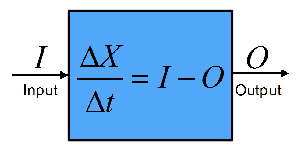
Figure B1.1: Illustration of the budget equation. A box containing a conserved quantity X that does not include internal sources or sinks will change in time according to the external inputs minus the outputs.
Different boxes can be connected such that the output of one box becomes the input of another box.
A budget is in balance if the quantity X does not change in time. In this case ΔX = 0 and the input equals the output:
(B1.3) 
Let’s do a little example. Assume a student gets a monthly stipend of $1,000 and $400 from his/her parents. Those are the inputs to the student’s bank account in units of dollars per month I = $1,000/month + $400/month = $1,400/month. The outputs would be the student’s monthly expenses. Let’s say he/she pays $400 for tuition, $420 for rent, $390 for food, and $100 for books (not for this one though) such that O = $400/month + $420/month + $390/month + $100/month = $1,310/month. The rate-of-change of his/her bank account is ΔX/Δt = I – O = $1,400/month – $1,310/month = $90/month. The student saves $90 per month.
Equation B1.2 can be used to predict the quantity X at time t2
(B1.4) 
from its value X1 at time t1 if the inputs and outputs are known. In climate modeling this method, called forward modeling, is used to predict quantities into the future one time step Δt at a time.
In our example, if the student starts at time t1, let’s say in January, with X1= $330 in his/her bank account then we can predict that in February he/she will have X2 = $330 + ($1,400/month – $1,310/month)×(1 month) = $330 + $90 = $420. Note that in this case the time step Δt = 1 month.
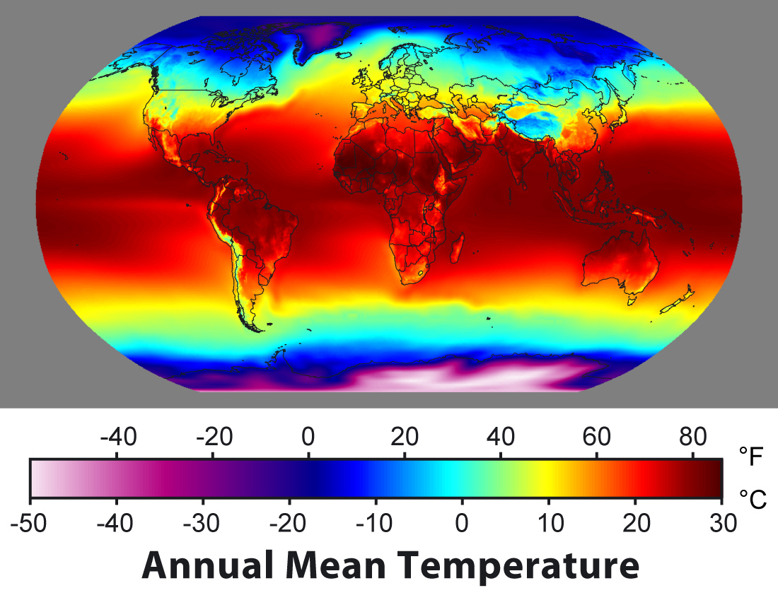
Earth’s energy budget is determined by energy input from the sun (solar radiation) and energy loss to space by thermal or terrestrial radiation, which is emitted from Earth itself. Solar radiation has shorter wavelengths than terrestrial radiation because the sun is hotter than Earth. To understand this let’s consider the electromagnetic radiation spectrum (Fig. 1). Electromagnetic radiation are waves of electric and magnetic fields that can travel through vacuum and matter (e.g. air) at the speed of light (c). It is one way that energy can be transferred from one place to another. The wavelength of electromagnetic radiation (λ), which is the distance from one peak to the next, varies by more than 16 orders of magnitude. Visible light, which has wavelengths from about 400 nm (nanometers, 1 nm = 10-9 m = one millionth of a millimeter) to about 700 nm, occupies only a small part of the entire spectrum of electromagnetic radiation. The frequency (ν) times the wavelength equals the speed of light c = νλ.
Albert Einstein showed in 1905 that electromagnetic radiation has particle properties. In modern quantum physics the light particle is called a photon. Each photon has a discrete amount of energy E = hv = hc/λ that corresponds to its wavelength, where h = 6.63×10⁻³⁴ Js is Planck’s constant. The shorter the wavelength the higher the energy. High energy photons at ultraviolet, X-ray, and gamma ray wavelengths can be harmful to biological organisms because they can destroy organic molecules such as DNA.

Figure 1: The Spectrum of Electromagnetic Radiation. Electromagnetic radiation ranges from radio-waves with wavelengths of hundreds of meters and more, to gamma rays, with wavelengths of 10-12 m, which is as small as the size of an atomic nucleus.
Interaction of electromagnetic radiation with matter depends on the wavelength of the radiation. Molecules have different discrete energy states and they can transition from one state to another one by absorbing or emitting a photon at a wavelength that corresponds to that energy difference (Fig. 2). Absorption (capture) of a photon leads to a transition from a lower to a higher energy state. Note that once absorbed the photon is gone and its energy has been added to the molecule. Emission (release) of a photon leads to a transition from a higher to a lower state (reversing the direction of the arrows in the top panel of Fig. 2). Note that the emitted photon can have a different wavelength that the absorbed photon. If, e.g., a UV photon was absorbed and has caused the energy of the molecule to increase from the ground electronic state to the second excited state, the molecule can emit two visible photons, first one that leads to a transition from the second to the first excited electronic state, and then another that leads to a transition to the ground state.
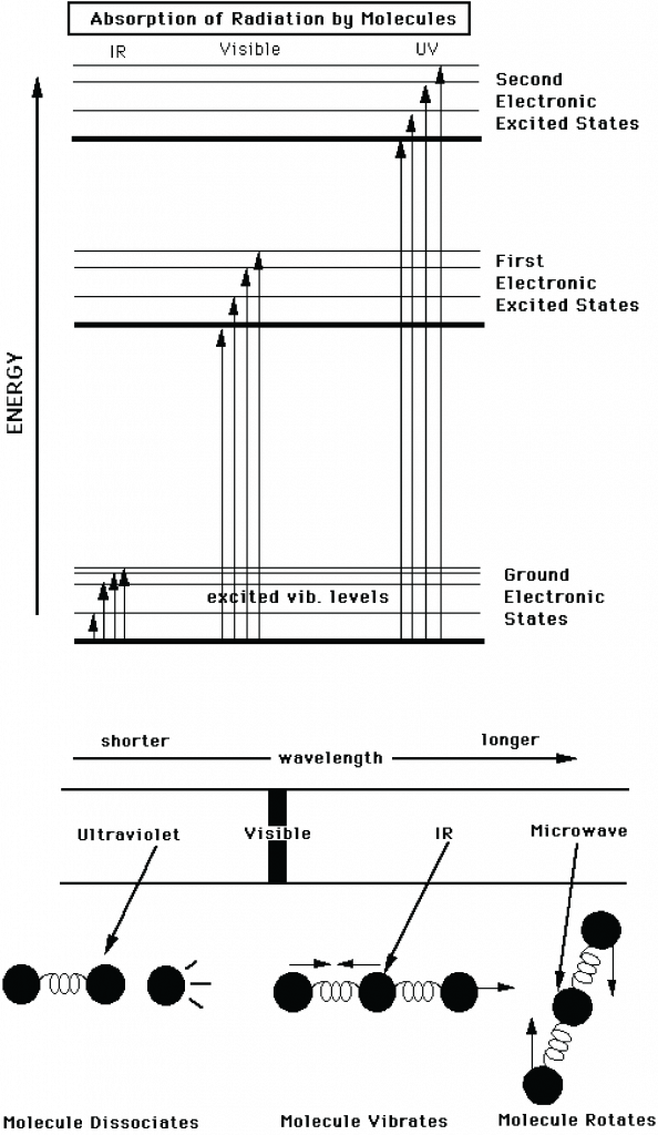
Figure 2: Interactions of electromagnetic radiation with molecules. Top: Absorption of a high-energy photon with an ultraviolet or visible wavelength can lead to excited electronic states. Each excited electronic energy state has sub-states with different vibrational levels. Absorption of a lower energy, infrared photon can excite a vibrational level without changing the electronic state. Bottom: Absorption of low-energy photons at microwave or infrared wavelengths can lead to rotation or vibration of molecules, whereas high-energy photons at ultraviolet wavelengths can break apart molecules. From
wag.caltech.edu.
In physics, a blackbody is an idealized object that can absorb and emit radiation at all frequencies. A blackbody emits radiation according to Planck’s law (Fig. 3). In classical physics experiments, a closed box covered on the inside with graphite is used to study its properties. It has only a small hole as an opening to measure the radiation that comes out of the box. Although a blackbody is an idealization many objects behave like a blackbody. Even fresh snow. Or the sun.
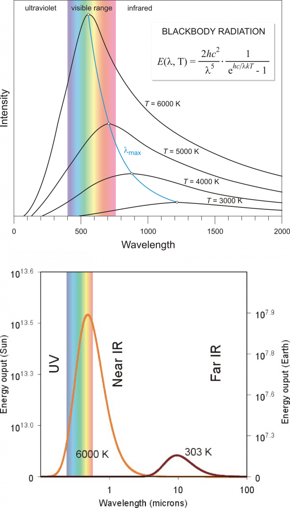
Figure 3: The intensity of blackbody radiation (arbitrary units) according to Planck’s law as a function of its wavelength (in nm in the top panel and μm (micrometers, 1 μm = 10
-6 m = 1,000 nm) in the bottom panel). The sun’s temperature is about 6,000 K, with a peak in the visible part of the spectrum. The blue curve in the top panel shows Wien’s law, which describes how the maximum moves towards larger wavelengths at colder temperatures. The bottom panel shows curves representative of sun’s (6,000 K) and Earth’s (303 K) temperatures. Note that the bottom panel uses a logarithmic x-axis and that the values for the sun (left scale) are about 6 orders of magnitude larger than those for Earth (right scale). Top image from
periodni.com, bottom image from
learningweather.psu.edu.
Integration of the Planck curve overall frequencies results in the Stefan-Boltzmann law
(1) 
which states that the total energy flux F in units of watts per square meter (Wm-2) emitted from an object is proportional to the absolute temperature of the object T in units of Kelvin (K) to the power four. The Stefan Boltzmann constant is σ = 5.67×10⁻⁸ Wm-2K-4 and ε is the emissivity (0 < ε < 1), a material-specific constant that allows for deviations from the ideal blackbody behavior (for which ε = 1). For ε = 1, F represents the area under the Planck curve. The emissivity for ice is 0.97, that for water is 0.96, and that for snow it is between 0.8 and 0.9. Thus, water and ice are almost perfect blackbodies, whereas for snow the approximation is less perfect but still good. Highly reflective materials such as polished silver (ε = 0.02) and aluminum foil (ε = 0.03) have low emissivities.
Equation (1) states that any object at a temperature larger than absolute zero emits energy. The energy emitted increases rapidly with temperature. E.g. a doubling of temperature will cause its radiative energy output to increase by a factor of 24 = 16.
Box 2: Earth’s Energy Balance Model 1 (Bare Rock)
A video element has been excluded from this version of the text. You can watch it online here: https://open.oregonstate.education/climatechange/?p=104
Figure B2.1: Illustration of the ‘Bare Rock’ Energy Balance Model. Yellow arrows indicate solar radiation. The red arrow represents terrestrial radiation.
We can now attempt to construct a simple model of the Earth’s energy budget in balance. The energy input is the absorbed solar radiation (ASR). The energy output is the emitted terrestrial radiation (ETR). Thus, equation B1.3 becomes
(B2.1) 
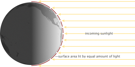
The absorbed solar radiation can be calculated from the total solar irradiance (TSI = 1,370 Wm-2), which is the flux of solar radiation through a plane perpendicular to the sun’s rays. (TSI is also sometimes called the solar constant although it is not constant but varies slightly as we’ll see below.) Since Earth is a rotating sphere the amount of radiation received per area is S = TSI/4 = 342 Wm-2 because the area of a sphere is 4 times the area of a disc with the same radius.
Part of the incident solar radiation is reflected to space by bright surfaces such as clouds or snow. This part is called albedo (a) or reflectivity. Earth’s average albedo is about a = 0.3. This means that one third of the incident solar radiation is reflected to space and does not contribute to heating the climate system. Therefore ASR = (1 – a) S = 240 Wm-2. Assuming Earth is a perfect blackbody ETR = σT4. With this equation B2.1 becomes
(B2.2) 
and we can solve for T = ((1 – a) S / σ)1/4. Inserting the above values for a, S, and σ gives T = 255 K or T = -18°C, suggesting Earth would completely freeze over as illustrated by ice sheets moving from the pole to the equator in the above animation. This is of course not what is going on in the real world and Earth’s actual average surface temperature, which is about 15°C, is much warmer. What’s wrong with this model? It is bare rock without an atmosphere! The model works well for planets without or with a very thin atmosphere like Mars, but it fails for planets that have thick atmospheres with gases that absorb infrared radiation such as Venus or Earth.
The concept of Earth’s energy balance goes back 200 years to French scientist Jean-Baptiste Fourier, as explained in this (1.5 h) documentary (discussion of Fourier’s contributions start at 9:52).
Temperature is the macroscopic expression of the molecular motions in a substance. In any substance such as the ideal gas depicted in Fig. 4 molecules are constantly in motion. They bump into each other and thus exchange energy. A single molecule is sometimes slow and at other times fast, but it is their average velocity that determines the temperature of a gas. More precisely, the temperature of an ideal gas T ~ E is proportional to the average kinetic energy  of its molecules. The faster they move the higher the temperature. At absolute zero temperature T = 0 K all motions would cease.
Figure 4: Animation of molecular motions in an ideal gas. From
en.wikipedia.org.
The lower panel in Fig. (3) shows blackbody curves for temperatures representative of the sun and Earth. Due to Earth’s lower temperature the peak in the radiation occurs at longer wavelengths around 10 μm in the infrared part of the spectrum. The sun’s radiation peaks around 0.5 μm in the visible part of the spectrum, but it also emits radiation at ultra-violet and near infrared wavelengths. Sunlight at the top-of-the-atmosphere is almost perfectly described by a blackbody curve (Fig. 5). Some solar radiation is absorbed by gases in the atmosphere but most is transmitted.
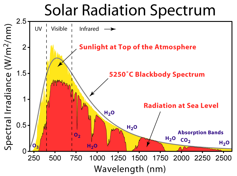
Figure 5. Solar radiation spectra for the incident sunlight at the top-of-the-atmosphere (yellow), at sea level (red), and a blackbody curve (grey). From
en.wikipedia.org.
Absorption by water vapor in the infrared and by ozone (O3) in the ultraviolet and scattering of light remove 25-30% of solar radiation before it hits the surface (Fig. 6). For Earth’s radiation, on the other hand, total absorption is with 70-85% much larger. The most important absorbers in the infrared are water vapor and CO2 whereas oxygen/ozone, methane, and nitrous oxide absorb smaller amounts. Gases that absorb infrared radiation are called greenhouse gases. There is only a relatively narrow window around 10 μm through which Earth’s atmosphere allows radiation to pass without much absorption. Thus, Earth’s atmosphere is mostly transparent to solar radiation, whereas it is mostly opaque to terrestrial radiation.
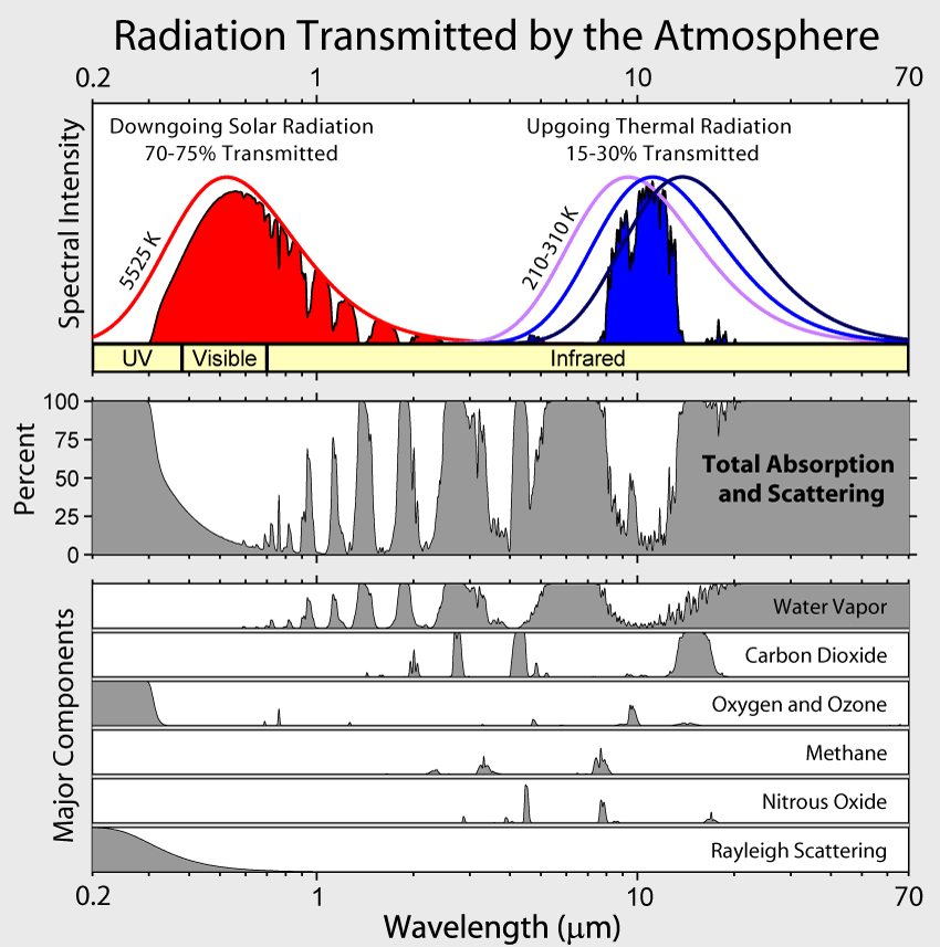
Figure 6: Radiation transmitted and absorbed by the cloud-free atmosphere. The left part of the figure shows the solar radiation and the right part shows Earth’s radiation. The blackbody curve at 5525 K (red curve in the top panel) represents the incident (downgoing) solar radiation at the top-of-the-atmosphere. The red filled area is the radiation transmitted through the atmosphere. The difference between the two (the white area between the red curve and the red area) is the amount absorbed by the atmosphere. For Earth’s radiation blackbody curves are shown for three temperatures (210, 260, and 310 K) and represent upgoing radiation from the surface. This is a key figure. From
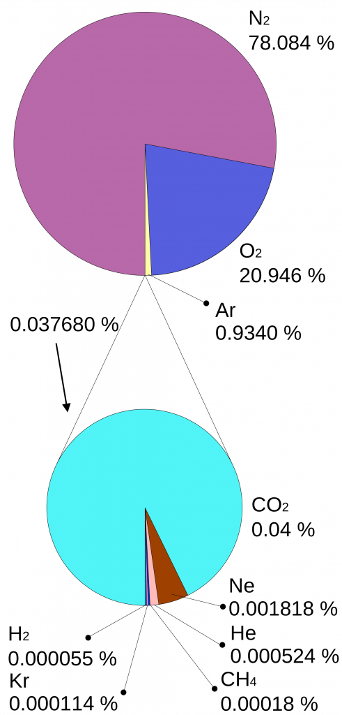
commons.wikimedia.orgWhy is it that only certain gases in the atmosphere absorb infrared radiation? After all there is much more nitrogen (N2) and oxygen (O2) gas in the atmosphere than water vapor and CO2 (Fig. 7). However, nitrogen and oxygen gas both consist of two atoms of the same element. Therefore, they do not have an electric dipole moment, which is critical for the interaction with electromagnetic radiation. Gas molecules that consist of different elements like water or CO2, on the other hand, do have dipole moments and can interact with electromagnetic radiation. Since CO2 is a linear and symmetric molecule it does not have a permanent dipole moment. However, during certain vibrational modes (Fig. 7) it attains a dipole moment and can absorb and emit infrared radiation. Detailed spectroscopic measurements of absorption coefficients show thousands of individual peaks in the spectra for water vapor and CO2 caused by the interaction of vibrational with rotational modes and broadening of lines by collisions (e.g. Pierrehumbert, 2011). These data are used by detailed, line-by-line radiative transfer models to simulate atmospheric transmission, absorption, and emission of radiation at individual wavelengths.
Figure 7:
Left: Composition of the dry atmosphere. Water vapor, which is not included in the image, varies widely but on average makes up about 1 % of the troposphere.
Top right: Vibrational modes of CO2. The black circles in the center represent the carbon atom, which carries a positive charge, whereas the oxygen atoms (white) carry negative charges. The asymmetric stretch mode (b) and the bend mode (c) lead to an electrical dipole moment, whereas the symmetrical stretch (a) does not. Modes (b) and (c) correspond to absorption peaks around 4 and 15 μm, respectively (Fig. 6).
Bottom right: Vibrational modes of H2O. The red balls in the center represent the negatively charged oxygen atom, whereas the white balls represent the positively charged hydrogen atoms. Due to its angle, it has a permanent dipole moment and various modes of vibration and rotation.
 |
 |
 |
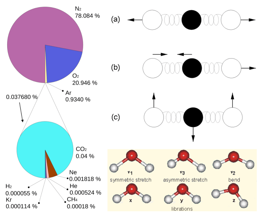
Figure 7:
Left: Composition of the dry atmosphere. Water vapor, which is not included in the image, varies widely but on average makes up about 1 % of the troposphere.
Top right: Vibrational modes of CO2. The black circles in the center represent the carbon atom, which carries a positive charge, whereas the oxygen atoms (white) carry negative charges. The asymmetric stretch mode (b) and the bend mode (c) lead to an electrical dipole moment, whereas the symmetrical stretch (a) does not. Modes (b) and (c) correspond to absorption peaks around 4 and 15 μm, respectively (Fig. 6).
Bottom right: Vibrational modes of H2O. The red balls in the center represent the negatively charged oxygen atom, whereas the white balls represent the positively charged hydrogen atoms. Due to its angle, it has a permanent dipole moment and various modes of vibration and rotation.
Absorption (emission) of radiation by the atmosphere tends to increase (decrease) its temperature. At equilibrium the atmosphere will emit just as much energy as it absorbs, but it will emit radiation in all directions, half of which goes downward and increases the heat flux to the surface. This additional heat flux from the atmosphere warms the surface. This is the greenhouse effect.
An atmosphere in which only radiative heat fluxes are considered and that was perfectly transparent in the visible and perfectly absorbing in the infrared would result in a much warmer surface temperature than our current Earth (see Perfect Greenhouse Model box below). It can also be easily shown that adding more absorbing layers would further increase surface temperatures to Ts = (n + 1)1/4T1, where T1 = 255 K is the temperature of the top-most of n layers. For two layers Ts = 335 K and the intermediate atmospheric layer’s temperature is T2 = 303 K. This could be called the ‘Super Greenhouse Model’. Thus, even though no infrared radiation from the surface can escape to space already with one perfectly absorbing layer, adding more absorbing layers further increases surface temperatures because it insulates the surface further from the top, which will always be at 255 K. In atmospheric sciences, this process is called increasing the optical thickness of the atmosphere.
Box 3: Earth’s Energy Balance Model 2 (Perfect Greenhouse)
Since Earth’s atmosphere absorbs most terrestrial radiation emitted from the surface, we may want to modify our ‘Bare Rock’ Energy Balance Model by adding a perfectly absorbing atmosphere. As in the ‘Bare Rock’ model the energy balance at the top-of-the-atmosphere gives us the emission temperature of the planet, which we now interpret as the atmospheric temperature Ta = 255 K. We now have an additional equation for the atmospheric energy balance. At equilibrium, the total emitted terrestrial radiation from the atmosphere (two times ETRa = σTa4 since one ETRa goes downward and one goes upward) must equal the absorbed radiation coming from the surface (ETRs = σTs4). This gives us a surface temperature of Ts = 21/4Ta = 303 K, which is too warm compared with the real world.
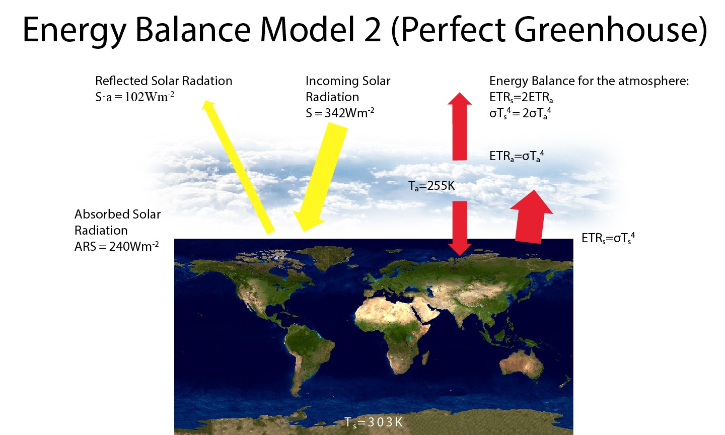
Figure B3.1: As Fig. B2.1 but for the ‘Perfect Greenhouse’ model.
In contrast to the ‘Perfect Greenhouse’ model, Earth’s atmosphere does absorb some solar radiation, it does transmit some infrared radiation, and, importantly, it is heated by non-radiative fluxes from the surface (Fig. 8). In fact, if only radiative fluxes (solar and terrestrial) are considered, surface temperatures turn out to be much warmer than they currently are and upper tropospheric temperatures are too cold (Manabe and Strickler, 1964). However, warming of the surface by absorbed solar and terrestrial radiation causes the air near the surface to warm and rise, causing convection. Convective motions cause both sensible and latent heat transfer from the surface to higher levels in the atmosphere. Most of this non-radiative heat transfer is in the form of latent heat. Evaporation cools the surface, whereas condensation warms the atmosphere aloft. Thus, the energy and water cycles on Earth are coupled.
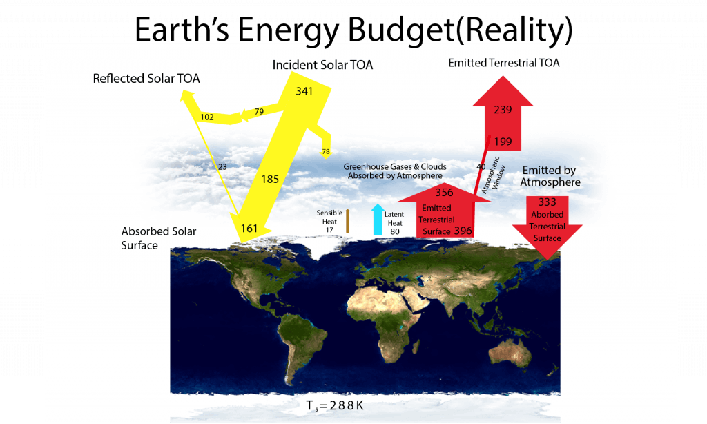
Figure 8: Earth’s energy budget estimated from modern observations and models. Adapted from Trenberth et al. (2009).
The downward terrestrial radiation from the atmosphere is the largest input of heat to the surface. In fact, it is more than twice as large as the absorbed solar radiation. This illustrates the important effect of greenhouse gases and clouds on the surface energy budget. The greenhouse effect is like a blanket that keeps us warm at night by reducing the heat loss. Similarly, the glass of a greenhouse keeps temperatures from dropping at night.
Clouds are almost perfect absorbers and emitters of infrared radiation. Therefore, cloudy nights are usually warmer than clear-sky nights. The important effect of water vapor on the greenhouse effect can be experienced by camping in the desert. Night-time temperatures there often get very cold due to the reduced greenhouse effect in the dry, clear desert air.
We’ve seen how adding greenhouse gases to the atmosphere increases its optical thickness and further insulates the surface from the top, which will lead to warming of the surface. But how much will it warm for a given increase in CO2 or another greenhouse gas? To answer this question and because we also want to consider other drivers of climate change we introduce the concepts of radiative forcing and feedbacks. These concepts are a way to separate different mechanisms that result in climate change. Radiative forcing is the initial response of radiative fluxes at the top-of-the-atmosphere. It can be defined as the change in the radiative balance at the top-of-the-atmosphere (the tropopause) for a given change in one specific process that affects those fluxes with everything else held constant. Examples for such a process are changes in greenhouse gas concentrations, aerosols, or solar irradiance.
A change in the radiative balance at the top-of-the-atmosphere will cause warming if the forcing is positive (more absorbed solar radiation or less emitted terrestrial radiation), and it will cause cooling if the forcing is negative (less absorbed solar or more emitted terrestrial to space). The amount of the resulting warming or cooling will not only depend on the strength of the forcing but also on feedback processes within the climate system. A climate feedback is a process that amplifies (positive feedback) or dampens (negative) the initial temperature response to a given forcing. E.g. as a response to increasing CO2 concentrations surface temperatures will warm, which will cause more evaporation and increased water vapor in the atmosphere. Since water vapor is also a greenhouse gas, this will lead to additional warming. Thus, the water vapor feedback is positive. The warming or cooling resulting from one specific forcing and all feedback processes is called climate sensitivity. Let’s discuss some of the known radiative forcings and feedback processes in more detail.
Radiative Forcings
Detailed radiative transfer models can be used to calculate the radiative forcing for changes in atmospheric greenhouse gas concentrations. As shown in Fig. (9) for CO2, the forcing turns out to depend logarithmically on its concentration (Ramaswamy et al., 2001)
(2) ![\begin{equation*} \Delta F = 5.35 [\mathrm{Wm^{-2}}] \ln (C / C_{0}), \end{equation*}](/books/PG441/images/000185.png "Rendered by QuickLaTeX.com")
where C is the CO2 concentration and C0 is the CO2 concentration of a reference state (e.g. the pre-industrial).
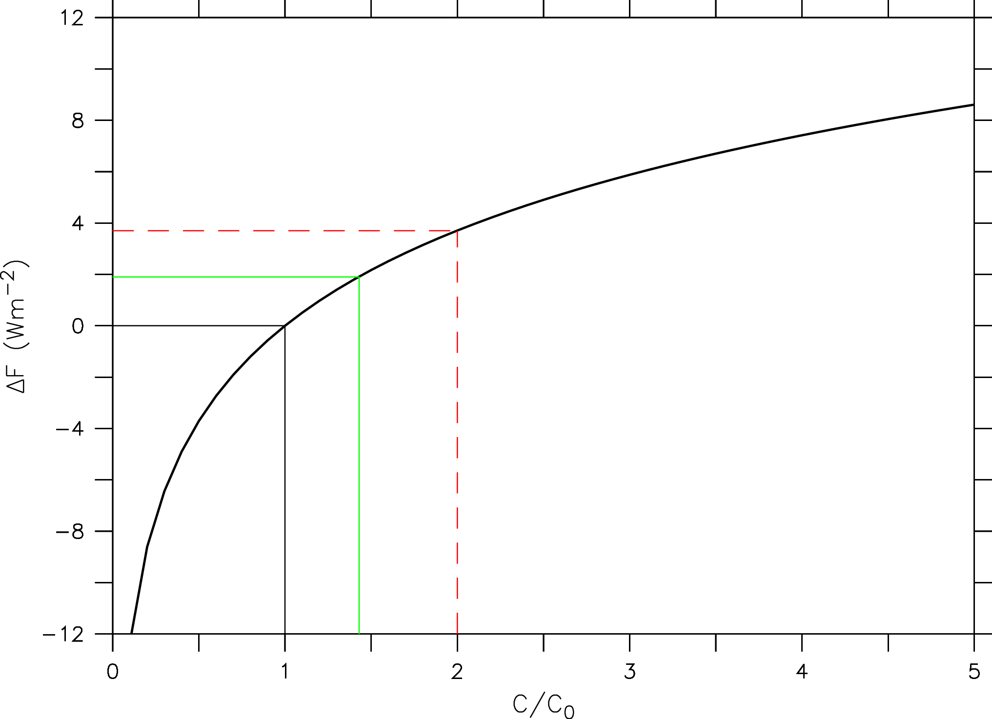
Figure 9: Radiative forcing (ΔF) in watts per square meter as a function of the atmospheric CO2 concentration (C) relative to a reference value (C0 ) according to eq. (2; black thick line). The black straight lines indicate the reference state C = C0 (ΔF = 0). The green and red dashed lines indicate the current (2016) state relative to the pre-industrial C/C0 = 400 ppm / 280 ppm = 1.4 (ΔF = 1.9 Wm-2) and that for a doubling of CO2 (ΔF2x = 3.7 Wm-2) respectively.
This means that the radiative effect of adding a certain amount of CO2 to the atmosphere will be smaller the more CO2 is already in the atmosphere. The reason for this is the saturation of peaks in the absorption spectrum (Fig. 6). E.g. in the center of the peak at 15 mm all radiation from the surface is already fully absorbed. Increasing CO2 further only broadens the width of the peak.
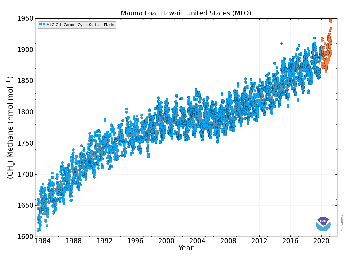
Figure 10: Top: Atmospheric methane concentrations as a function of time. Top: Recent air measurements from Mauna Loa.
Bottom: Ice core, firn, and air measurements from Antarctica. Note that most methane sources are in the northern hemisphere, which leads to higher concentrations there compared with the southern hemisphere.
 |
 |
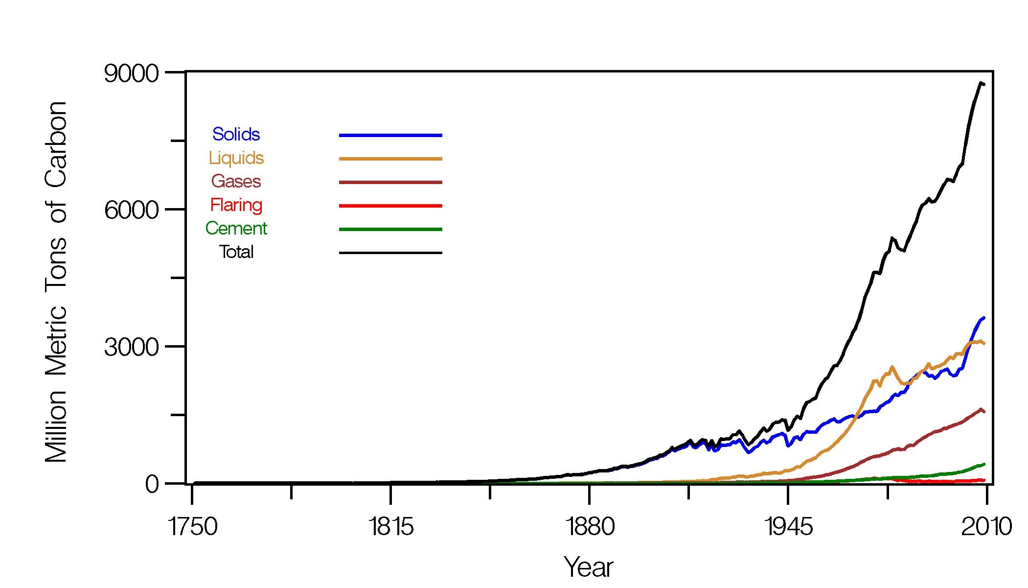
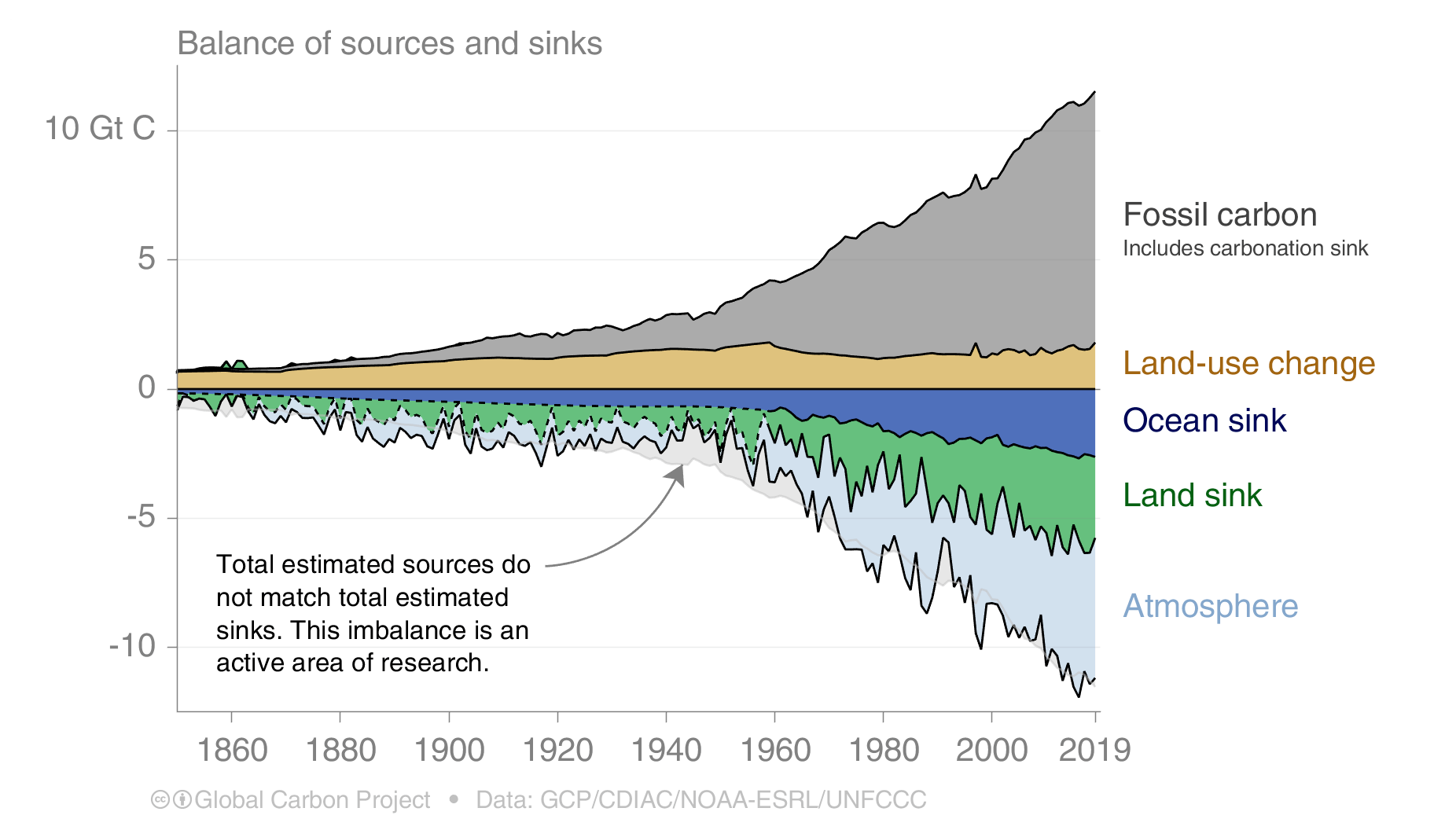
Methane (CH4) is produced naturally in wetlands and by various human activities such as in the energy industry, in rice paddies, and by agriculture (e.g. cows). It is removed by chemical reaction with OH radicals and has a lifetime of about 10 years. Anthropogenic activities have increased atmospheric methane concentrations since the industrial revolution by more than a factor of two, from around 700 ppb to more than 1600 ppb currently (Fig. 10). On a per-molecule basis methane is a much more potent greenhouse gas than CO2, perhaps in part because its main absorption peak around 8 mm is less saturated than the one for CO2 (Fig. 6). However, since methane concentrations are more than two orders of magnitude smaller than CO2 concentrations, its radiative forcing since the industrial revolution is 0.5 Wm-2, which is less than that for CO2. As we will see below CO2 also has a much longer lifetime than methane and therefore it can accumulate over long timescales. Indeed, while recent measurements indicate a slowdown of methane growth rates in the atmosphere, CO2 increases at ever higher rates (Fig. 8 in Chapter 2).
Aerosols are small particles suspended in the air. Natural processes that deliver aerosols into the atmosphere are dust storms and volcanic eruptions. Burning of oil and coal by humans also releases aerosols into the atmosphere. Aerosols have two main effects on Earth’s radiative balance. They directly reflect sunlight back to space (direct effect). They also act as cloud condensation nuclei such that they can cause more or brighter clouds, which also reflect more solar radiation back to space. Thus, both the direct and indirect effects of increased aerosols lead to cooling of the surface. Therefore, aerosol forcing is negative.
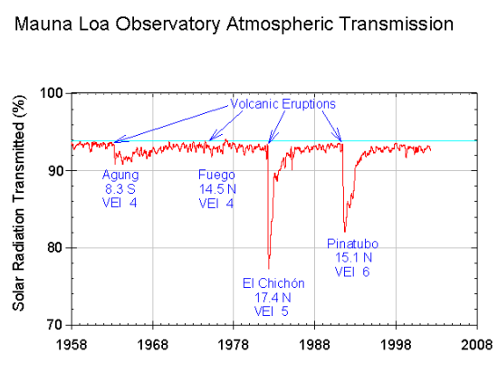
Large explosive volcanic eruptions can lead to ash particles and gas such as sulfur dioxide (SO2) ejected into the stratosphere, where they can be rapidly distributed over large areas (Fig. 11). In the stratosphere SO2 is oxidized to form sulfuric acid aerosols. However, stratospheric aerosols eventually get mixed back into the troposphere and removed through precipitation or dry deposition. The lifetime of volcanic aerosols in the stratosphere is in the order of months to a few years. Estimates of the radiative forcing from volcanic eruptions depend on the eruption but varies from a few negative tenths of a watt per square meter to -3 or -4 Wm-2 for the largest eruptions during the last 100 years (Fig. 12).
Figure 11: Effects of volcanic eruptions.
Top: Measurements of solar radiation transmitted at Hawaii’s Mauna Loa Observatory.
Center: Photograph of a rising Pinatubo ash plume.
Bottom: Photograph from Space Shuttle over South America taken on Aug. 8, 1991 showing the dispersion of the aerosols from the Pinatubo eruption in two layers in the stratosphere above the top of cumulonimbus clouds.
 |
 |
 |
Anthropogenic aerosols are released from burning tropical forests and fossil fuels. The latter is the major component producing more sulfate aerosols currently than those naturally produced. Aerosol concentrations are higher in the northern hemisphere, where industrial activity is located. Radiative forcing estimates are uncertain but vary between about -0.5 to -1.5 Wm-2 for both direct and indirect effects (Figs. 12, 13). Generally, estimates of aerosol forcings are more uncertain than those for greenhouse gases.
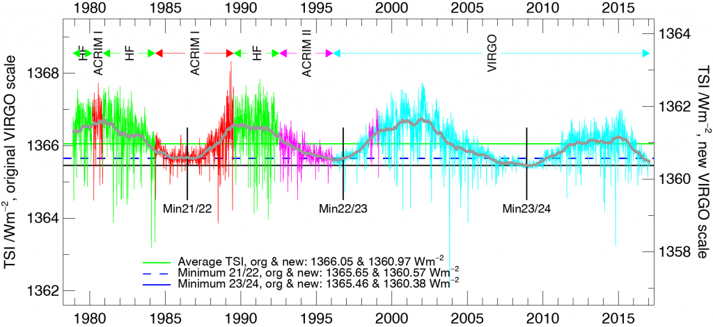
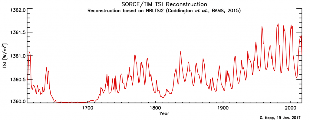
Solar irradiance varies with the 11-year sunspot cycle. Direct, satellite-based observations of total solar irradiance show variations of about 1 Wm-2 between sunspot maxima and minima (Fig. 14). To estimate radiative forcing TSI needs to be divided by four, which results in about 0.25 Wm-2. Longer-term estimates of TSI variations based on sunspot cycles indicate an increase from the Maunder Minimum (1645-1715) to the present by about 1 Wm-2. The resulting forcing is again about 0.25 Wm-2.
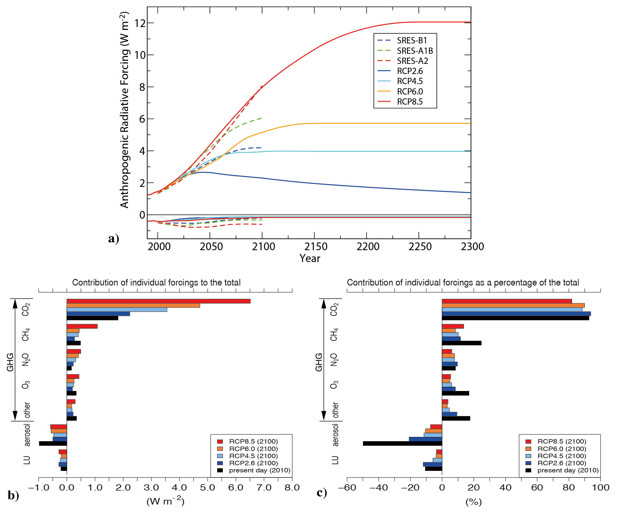
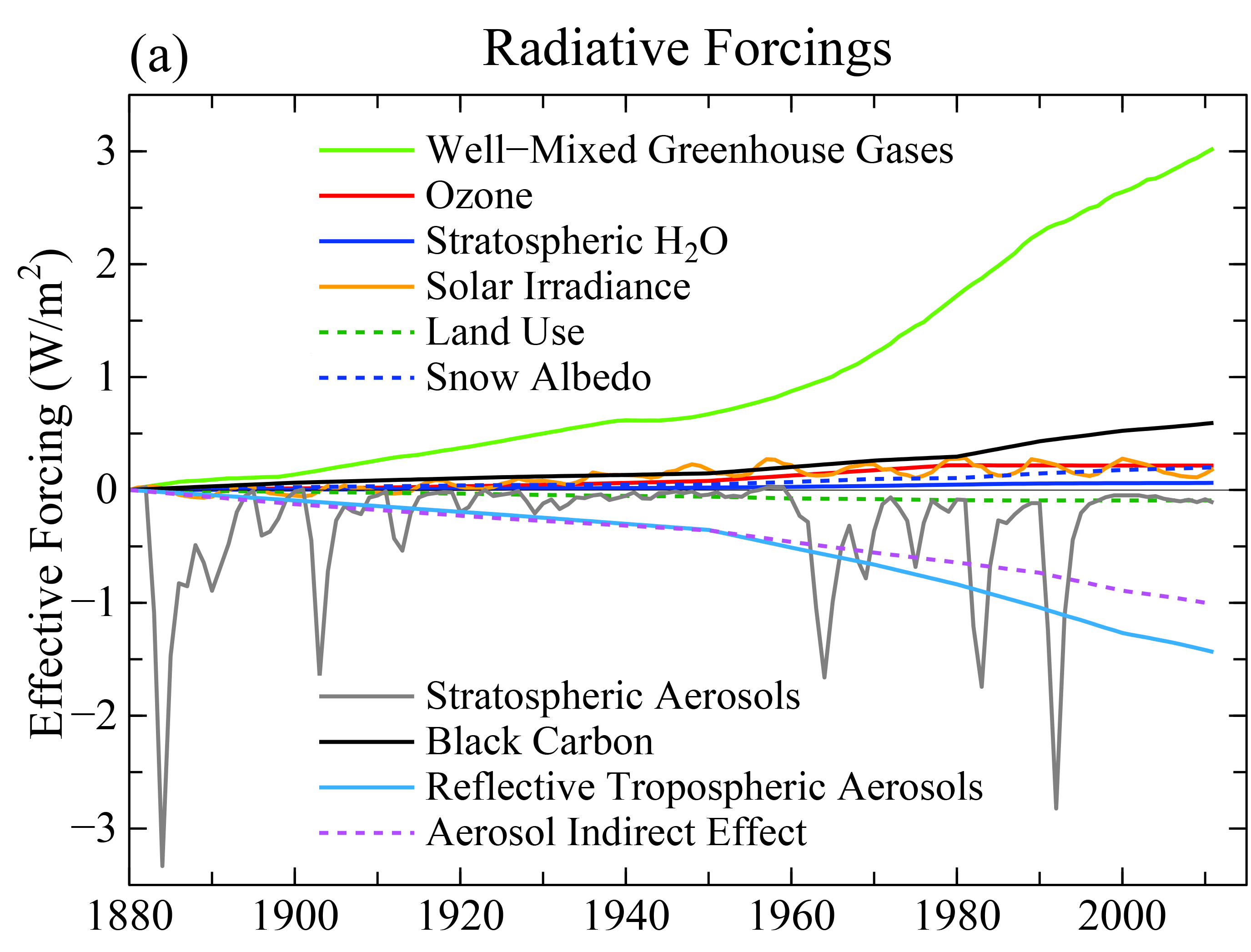
Comparisons of the different forcings indicate that long-term trends of the last 100 years or so are dominated by anthropogenic forcings. The negative forcings from increases in aerosols compensate somewhat the positive forcings from the increase in greenhouse gases. However, the net effect is still a positive forcing of about 2 Wm-2. Volcanic forcings are episodic and the estimates of solar forcing are much smaller than those of anthropogenic forcings.
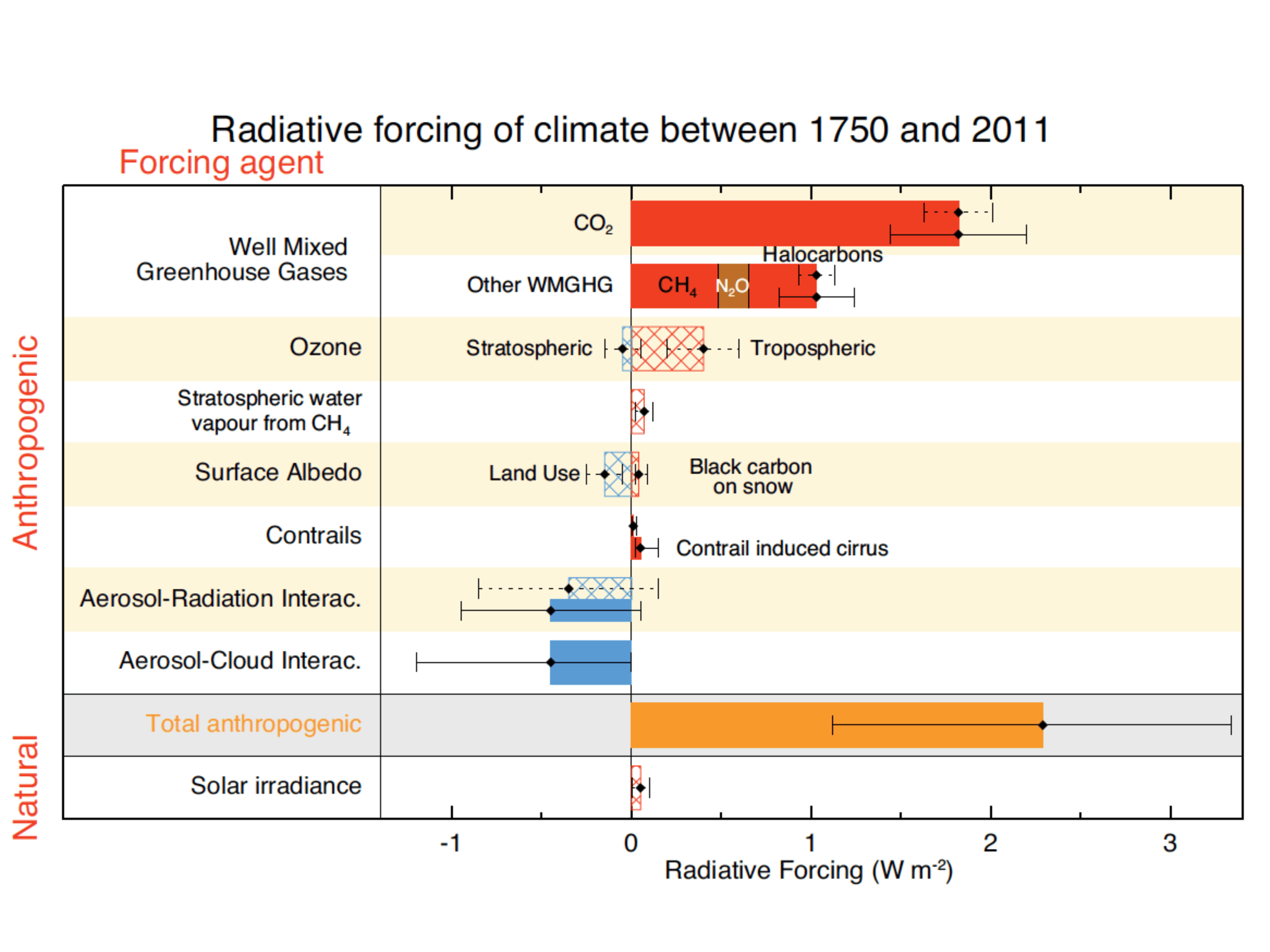
Figure 13: Summary of radiative forcings. From IPCC (2013). Hatched bars denote low confidence and scientific understanding.
Figure 14: Total solar irradiance variations.
Top: measurements based on various satellites as a function of time.
Bottom: longer term reconstructions.
 |
 |
Feedback Processes
A feedback process is a modifier of climate change. It can be defined as a process that can amplify or dampen the response to the initial radiative forcing through a feedback loop. In a feedback loop the output of a process is used to modify the input (Fig. 15). By definition, a positive feedback amplifies and a negative feedback dampens the response. In our case, the input is the radiative forcing (ΔF) and the output is the global average temperature change (ΔT).
Figure 15: Schematic illustration of fast climate feedback loops (left) and their effects on the vertical temperature distribution in the troposphere (right).
A video element has been excluded from this version of the text. You can watch it online here: https://open.oregonstate.education/climatechange/?p=104
|
Imagine talking into a microphone. A positive feedback process works like the amplifier that makes your voice louder. It can lead to a runaway effect if no or only weak negative feedback processes are present. If you hold the microphone too close to the speaker, the runaway effect can result in a loud noise. Early in Earth’s history, between about 500 million and 1 billion years ago, Earth may have experienced a runaway effect into a completely ice and snow covered planet called ‘Snowball Earth’ caused by the ice-albedo feedback (see below). An example of a negative feedback process would be talking into a pillow. This makes your voice quieter. A negative feedback is stabilizing. It prevents a runaway effect. Both positive and negative feedback processes operate in the climate system. (Try to imagine talking into multiple pillows and microphones.) In the following we will discuss the most important ones.
Let’s assume we have an initial positive forcing (ΔF > 0) as illustrated in Fig. 15. As a response, temperatures in the troposphere will warm. Since the troposphere is well mixed, we can assume that the warming is uniform (ΔTs = ΔTa > 0). Thus, the upper troposphere will warm, which will lead to increased emitted terrestrial radiation (ΔETRa > 0) to space. Increased heat loss opposes the forcing and leads to cooling. This is the Planck feedback, and it is negative. Equilibrium will be achieved if ΔETRa = ΔF. Since ΔETRa = ETRa,f–ETRa,i is the difference between the final ETRa,f = σ(Ta + ΔTa)4 and the initial ETRa,i = 240 Wm-2 as calculated above (e.g. Fig. B2.1), we can calculate the surface temperature change due to the forcing and the Planck feedback ΔTpl = ΔTa = [(ETRa,i + ΔF)/σ]1/4 – Ta. For a doubling of atmospheric CO2 ΔF = 3.7 Wm-2 this results in ΔTpl = 1 K.
Thus, if only the Planck feedback was operating and everything else would be fixed, a doubling of CO2 would result in a warming of about 1 K. However, warmer air and surface ocean temperatures will also lead to more evaporation. The amount of water vapor an air parcel can hold depends exponentially on its temperature. This relationship, which can be derived from classical thermodynamics, is called the Clausius-Clapeyron relation (Fig. 16). Since most of Earth is covered in oceans there is no lack of water available for evaporation. Therefore, it is likely that warmer air temperatures will lead to more water vapor in the atmosphere. Because water vapor is a strong greenhouse gas this will lead to an additional reduction in the amount of outgoing longwave radiation and therefore to more warming. Thus, the water vapor feedback is positive. If we assume again that the temperature change is uniform with height the troposphere will warm by an additional amount ΔTwv due to the water vapor feedback (red line in Fig. 15).
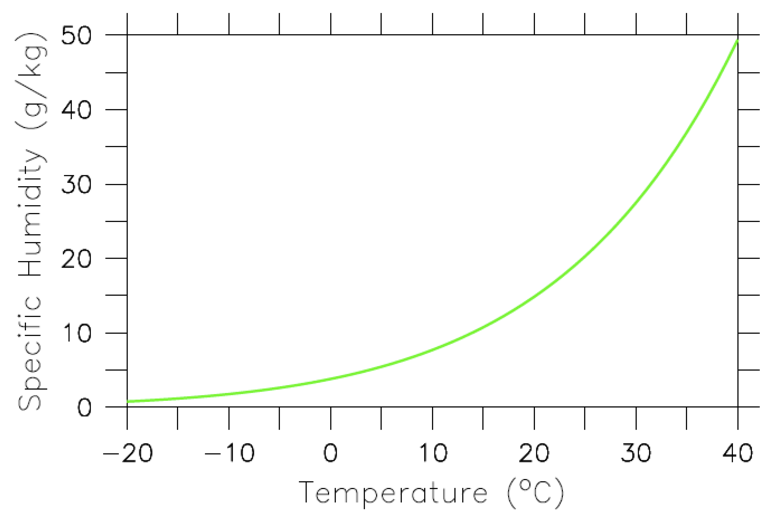
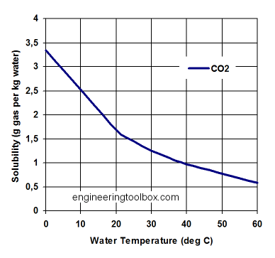
Figure 16: The Clausius-Clapeyron relation describes the amount of water vapor (in g water per kg of moist air) that air at saturation can hold as a function of temperature. The water-holding capacity of air increases approximately exponentially with temperature such that a 1 degree C warming leads to a 7% increase in humidity. All points long the green line represent 100% relative humidity. The lower a point is below the green line the lower its relative humidity will be. E.g. a point half way between the green line and the zero line would have 50% relative humidity.
Increased amounts of water vapor in the atmosphere also imply increased vertical transport of water vapor and thus more latent heat release at higher altitudes where condensation occurs. This warms the air aloft ΔTlr > 0. In contrast, at the surface increased evaporation leads to cooling ΔTlr < 0. Thus, the lapse-rate, Γ = ΔT/Δz, which is the change in temperature with height in the atmosphere, is expected to decrease. Warming of the upper atmosphere will increase outgoing longwave radiation. Therefore, similarly to the Planck feedback, the lapse rate feedback is negative.
Since both the water vapor and the lapse rate feedback are caused by changes in the hydrologic cycle, they are coupled. This results in reduced uncertainties in climate models if the combined water vapor plus lapse rate feedback is considered rather than each feedback individually (Soden and Held, 2006).
Warming surface temperatures will also cause melting of snow and ice. This decreases the albedo and thus it increases the amount of absorbed solar radiation, which will lead to more warming. Thus, the ice-albedo feedback is positive. Our simple energy balance model 2 from above can be modified to include a temperature dependency of the albedo, which can exhibit a runaway transition to a snowball Earth and interesting hysteresis behavior. Hysteresis means that the state of a system does not only depend on its parameters but also on its history. Transitions between states can be rapid even if the forcing changes slowly.
Warming will also likely change clouds. However, no clearly understood mechanism has been identified so far that would make an unambiguous prediction how clouds would change in a warmer climate. Comprehensive climate models predict a large range of cloud feedbacks. Most of them are positive, but a negative feedback cannot be excluded at this point. The cloud feedback is the least well understood and the most uncertain element in climate models. It is also the source of the largest uncertainty for future climate projections.
Climate models can be used to quantify individual feedback parameters γi. They are calculated as the change in the radiative flux at the top-of-the-atmosphere ΔRi divided by the change of the controlling variable Δxi: γi = ΔRi/Δxi. E.g. to quantify the Planck feedback the controlling variable Δxi = ΔT is atmospheric temperature. The atmospheric temperature is increased everywhere by ΔT = 1 K and then the radiative transfer model calculates ΔR at every grid point of the model, that is at all latitudes and longitudes, and then averages over the whole globe. This results in ΔRpl and γpl = ΔRpl/ΔT. All individual feedback parameters can be added to yield the total feedback γ = γpl + γwv + γlr + γia + γcl. The total feedback has to be negative to avoid a runaway effect. The strongest, most precisely known feedback is the Planck feedback, which is about γpl = −3.2 Wm-2K-1. Estimates for the other feedbacks are about γwv + γlr ≅ +1 Wm-2K-1 for the combined water vapor / lapse rate feedbacks, γia = +0.3 Wm-2K-1 for ice-albedo feedback, and γcl = +0.8 Wm-2K-1 for the cloud feedback. This gives for the total feedback γ values from about −0.8 to about −1.6 Wm-2. The total feedback parameter can be used to calculate the climate sensitivity.
Climate Sensitivity
The climate sensitivity ΔT2× is usually defined as the global surface temperature change for a doubling of atmospheric CO2 at equilibrium and it includes all fast feedbacks discussed above. Current best estimates are ΔT2× ≅ 3 K, however it ranges from about 1.5 to about 4.5 K. This large uncertainty is mostly due to the large uncertainty of the cloud feedback. Sometimes the climate sensitivity SC = −1/γ is reported in units of K/(Wm-2). Since we know the forcing for a doubling of CO2 ΔF2× = 3.7 Wm-2 quite well, one can be calculated from the other using SC = ΔT2×/ΔF2×. For ΔT2× ≅ 3 K, SC ≅ 0.8 K/(Wm-2), and γ ≅ 1.2 Wm-2K-1. Note that slow feedbacks associated with the growth and melting of ice sheets or changes in the carbon cycle are not included in these numbers. Since we would expect those feedbacks to be also positive we can expect an even higher climate sensitivity for longer timescales (hundredths to thousandths of years).
Our definitions of radiative forcings and feedbacks above are not clear cut. They are based on existing climate models and the processes included in them. For example changes in atmospheric CO2 concentrations over long paleoclimate timescales can be thought of as a feedback rather than a forcing since the ultimate forcing of the ice age cycles are changes in the Earth’s orbital parameters and hence the seasonal distribution of solar radiation.


 is larger than the height of the equilibrium line HE the ice sheet is in a stable equilibrium. However, if warming temperatures rise the equilibrium line to
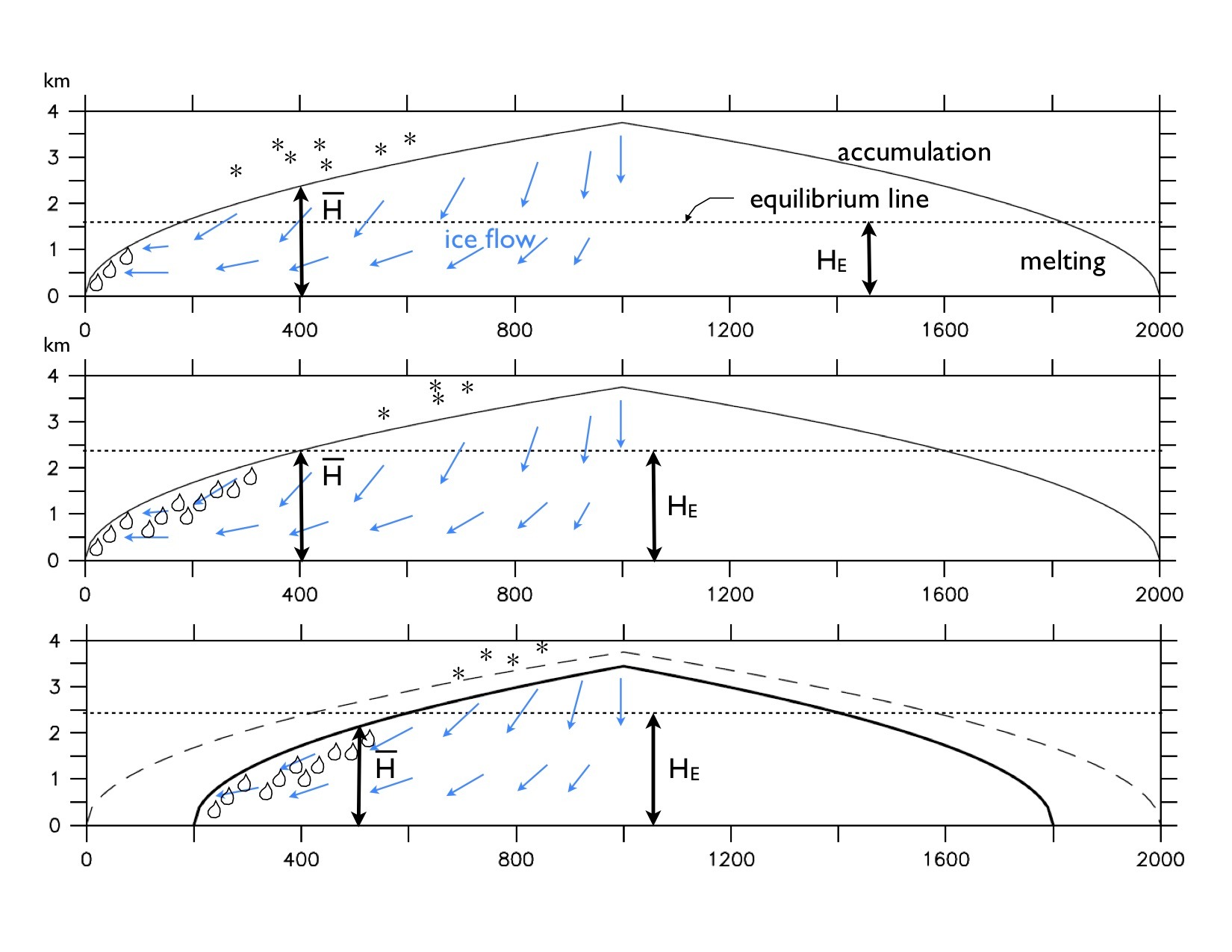


 . Some are a little faster, others are a little slower. Only the fastest will be able to leave the water phase and make it to the vapor phase (air). (
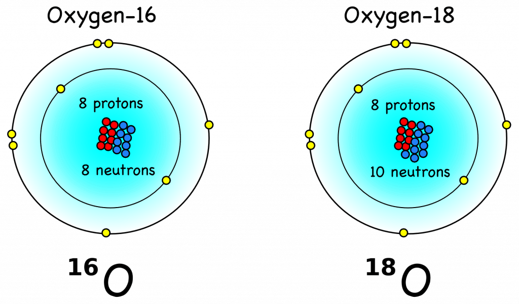
 , where R = 18O/16O is the heavy over light ratio of a sample, relative to that of a standard Rstd. Fig. B2 illustrates how fractionation during evaporation and condensation affects the isotope values of water, vapor, and ice in the global hydrological cycle.
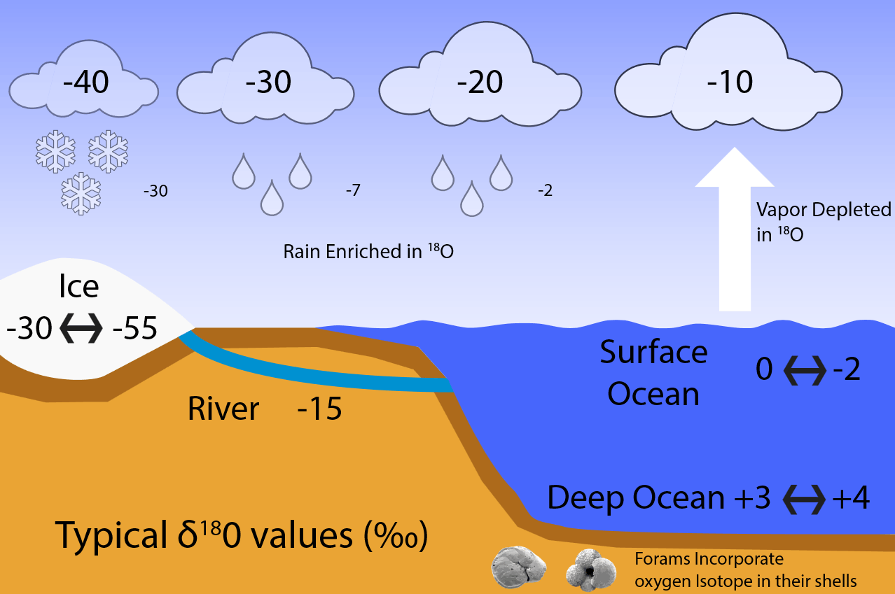
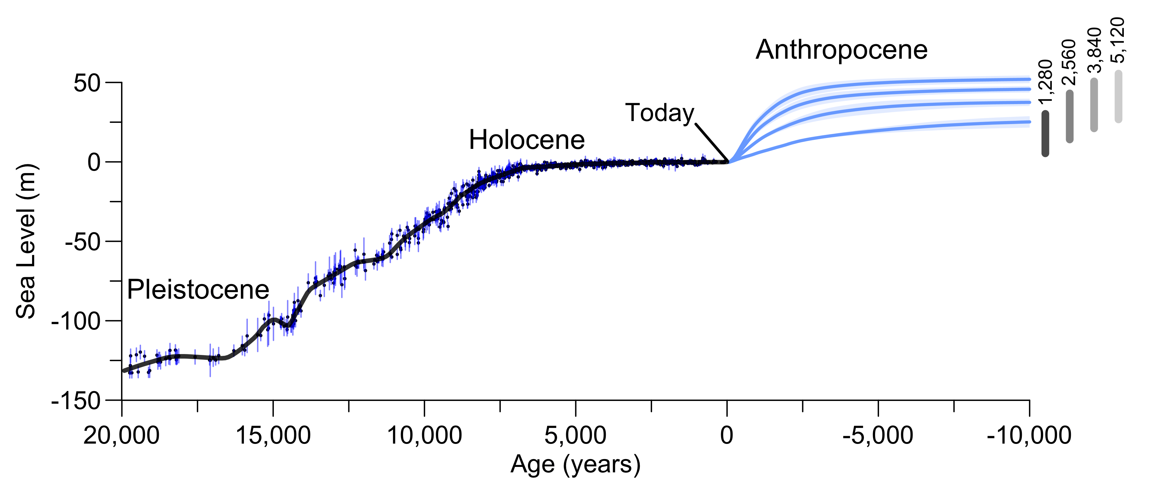
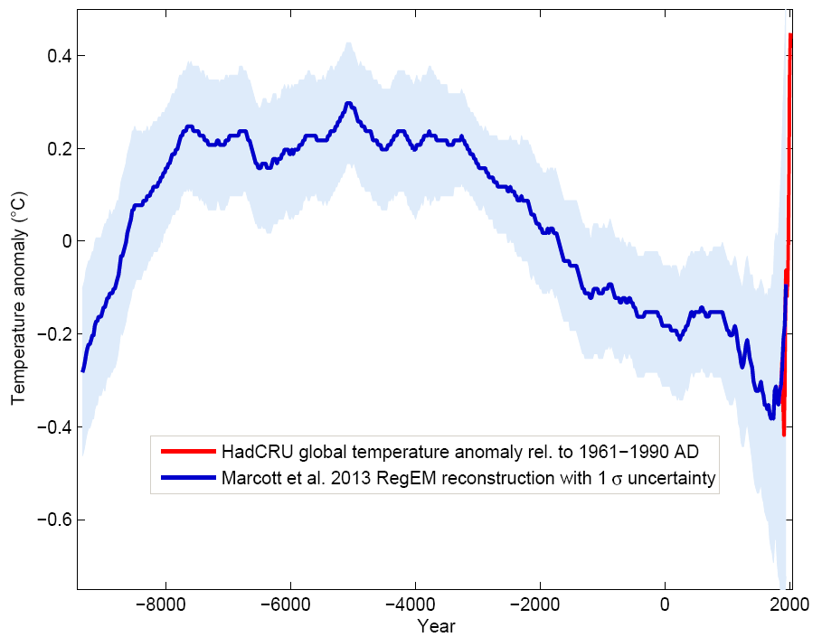
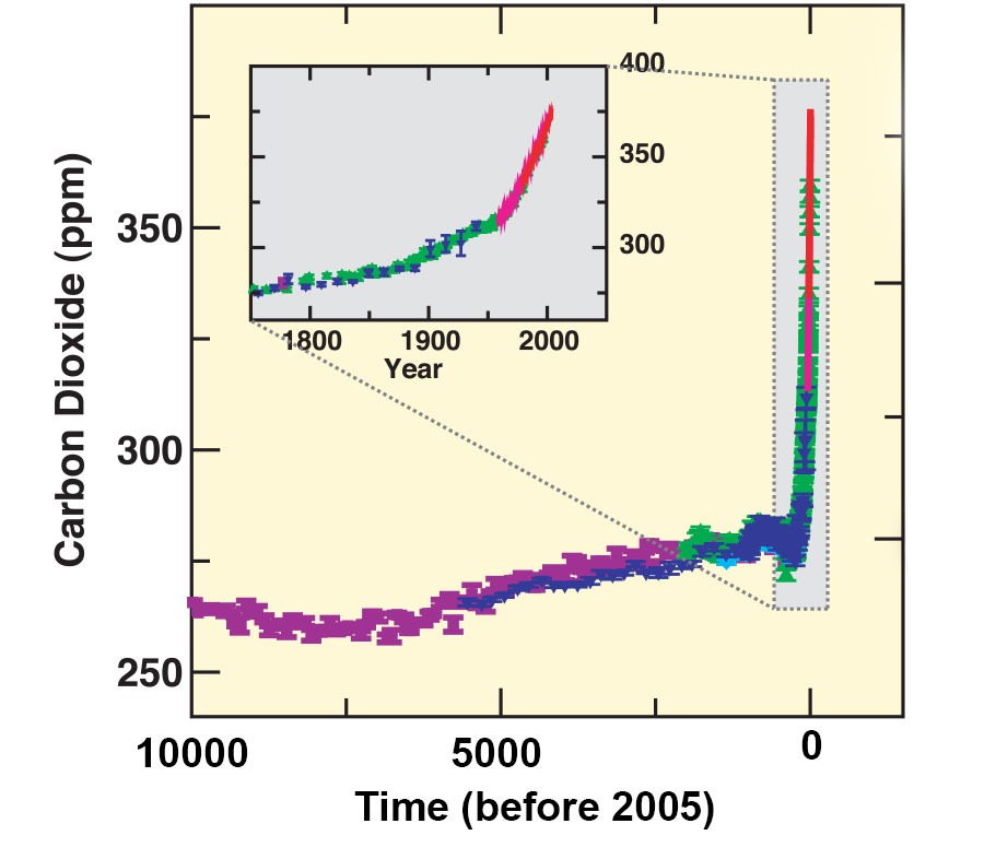
![Glacial-interglacial Cycles. Top: Antarctic temperature anomaly estimated from deuterium ratios measured in the ice (Jouzel et al., 2007). Deuterium (D) is the heavy hydrogen isotope 2H. In H2O it works similar to the heavy oxygen isotope as a local temperature proxy. Center: Atmospheric CO2 concentrations from ice cores (Lüthi et al., 2008). Bottom: Global sea level changes (ΔSL = [δ18O - 3.2 ‰]×[-120 m / 1.69 ‰]) estimated from oxygen isotopes (δ18O) measured in benthic foraminifera from deep-sea sediments (Lisiecki and Raymo, 2004). This is a key figure.](/books/PG441/images/000091.png)

